Revision as of 13:39, 2 December 2018

ChtMultiRegionFoam

   Solver for steady or transient fluid flow and solid heat conduction, with
   conjugate heat transfer between regions, buoyancy effects, turbulence,
   reactions and radiation modelling.

1 Equations

For each region defined as fluid, the according equation for the fluid is solved and the same is done for each solid region. The regions are coupled by a thermal boundary condition. A short description of the solver can be found also in ^[1]

1.1 Equations Fluid

For each fluid region the compressible Navier Stokes equation are solved.

1.1.1 Mass conservation

The variable-density continuity equation is

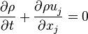\frac{\partial \rho}{\partial t} + \frac{\partial {\rho u}_j}{\partial x_j} = 0

(1)

The source code can be found in src/finiteVolume/cfdTools/compressible/rhoEqn.H:

 
 
{
    fvScalarMatrix rhoEqn
    (
        fvm::ddt(rho)
      + fvc::div(phi)
      ==
        fvOptions(rho)
    );
 
    fvOptions.constrain(rhoEqn);
 
    rhoEqn.solve();
 
    fvOptions.correct(rho);
}

1.1.2 Momentum conservation

\frac{ \partial (\rho {u}_i)}{\partial t} + \frac{\partial}{\partial x_j} \left( \rho {u}_j u_i \right) = - \frac{\partial p_{rgh}} {\partial{x_i}} - \frac{\partial \rho g_j x_j}{\partial x_i} + \frac{\partial}{\partial x_j} \left( \tau_{ij} + \tau_{t_{ij}} \right)

(2)

$u$ represent the velocity, $g_i$ the gravitational acceleration, 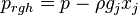$p_{rgh} = p - \rho g_j x_j$ the pressure minus the hydrostatic pressure and $\tau_{ij}$ and $\tau_{t_{ij}}$ are the viscose and turbulent stresses.

The source code can be found in Ueqn.H:

 
 
    // Solve the Momentum equation
 
    MRF.correctBoundaryVelocity(U);
 
    tmp<fvVectorMatrix> tUEqn
    (
        fvm::ddt(rho, U) + fvm::div(phi, U)
      + MRF.DDt(rho, U)
      + turbulence.divDevRhoReff(U)
     ==
        fvOptions(rho, U)
    );
    fvVectorMatrix& UEqn = tUEqn.ref();
 
    UEqn.relax();
 
    fvOptions.constrain(UEqn);
 
    if (pimple.momentumPredictor())
    {
        solve
        (
            UEqn
         ==
            fvc::reconstruct
            (
                (
                  - ghf*fvc::snGrad(rho)
                  - fvc::snGrad(p_rgh)
                )*mesh.magSf()
            )
        );
 
        fvOptions.correct(U);
        K = 0.5*magSqr(U);
    }
 
    fvOptions.correct(U);

1.1.3 Energy conservation

The energy equation can be found in: https://cfd.direct/openfoam/energy-equation/

The total energy of a fluid element can be seen as the sum of kinetic energy $k = 0.5 u_i u_i$ and internal energy $e$ . The rate of change of the kinetic energy within a fluid element is the work done on this fluid element by the viscous forces, the pressure and eternal volume forces like the gravity:

\frac{ \partial (\rho k)}{\partial t} + \frac{\partial}{\partial x_j} \left( \rho {u}_j k \right) = - \frac{\partial p u_j} {\partial{x_i} }- \rho g_j u_j + \frac{\partial}{\partial x_j}\left( \tau_{ij} u_i \right)

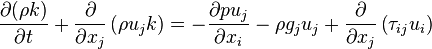(3)

The rate of change of the internal energy $e$ of a fluid element is the heat transferred to this fluid element by diffusion and turbulence $q_i + q_{ti}$ plus the heat source term $r$ plus the heat source by radiation $Rad$ :

\frac{ \partial (\rho e)}{\partial t} + \frac{\partial}{\partial x_j} \left( \rho {u}_j e \right) = - \frac{\partial q_i} {\partial{x_i} } + \rho r + Rad

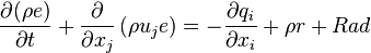(4)

The change rate of the total energy is the sum of the above two equations:

\frac{ \partial (\rho e)}{\partial t} + \frac{\partial}{\partial x_j} \left( \rho {u}_j e \right) + \frac{ \partial (\rho k)}{\partial t} + \frac{\partial}{\partial x_j} \left( \rho {u}_j k \right) = - \frac{\partial ( q_i + q_{ti}) } {\partial{x_i} } + \rho r + Rad - \frac{\partial p u_j} {\partial{x_i} }- \rho g_j u_j + \frac{\partial}{\partial x_j}\left( \tau_{ij} u_i \right)

(5)

Instead of the internal energy $e$ there is also the option to solve the equation for the enthalpy 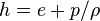$h = e + p/\rho$ :

\frac{ \partial (\rho h)}{\partial t} + \frac{\partial}{\partial x_j} \left( \rho {u}_j h \right) + \frac{ \partial (\rho k)}{\partial t} + \frac{\partial}{\partial x_j} \left( \rho {u}_j k \right) = - \frac{\partial ( q_i + q_{ti})} {\partial{x_i} } + \rho r + Rad + \frac{\partial p} {\partial{t} }- \rho g_j u_j + \frac{\partial}{\partial x_j}\left( \tau_{ij} u_i \right)

(5)

The source code can be found in EEqn.H:

 
{
    volScalarField& he = thermo.he();
 
    fvScalarMatrix EEqn
    (
        fvm::ddt(rho, he) + fvm::div(phi, he)
      + fvc::ddt(rho, K) + fvc::div(phi, K)
      + (
            he.name() == "e"
          ? fvc::div
            (
                fvc::absolute(phi/fvc::interpolate(rho), U),
                p,
                "div(phiv,p)"
            )
          : -dpdt
        )
      - fvm::laplacian(turbulence.alphaEff(), he)
     ==
        rho*(U&g)
      + rad.Sh(thermo, he)
      + Qdot
      + fvOptions(rho, he)
    );
 
    EEqn.relax();
 
    fvOptions.constrain(EEqn);
 
    EEqn.solve();
 
    fvOptions.correct(he);
 
    thermo.correct();
    rad.correct();
 
    Info<< "Min/max T:" << min(thermo.T()).value() << ' '
        << max(thermo.T()).value() << endl;
}

1.1.4 Species conservation

In order to account for the chemical reactions occurring between different chemical species a conservation equation for each species k has to be solved:

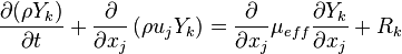\frac{ \partial (\rho Y_k)}{\partial t} + \frac{\partial}{\partial x_j} \left( \rho {u}_j Y_k \right) = \frac{\partial } {\partial{x_j} }\mu_{eff}\frac{\partial Y_k}{\partial x_j} + R_k

(6)

$R_k$ is the reaction rate of the species k.

The source code can be found in YEqn.H:

 
tmp<fv::convectionScheme<scalar>> mvConvection(nullptr);
 
if (Y.size())
{
    mvConvection = tmp<fv::convectionScheme<scalar>>
    (
        fv::convectionScheme<scalar>::New
        (
            mesh,
            fields,
            phi,
            mesh.divScheme("div(phi,Yi_h)")
        )
    );
}
 
{
    reaction.correct();
    Qdot = reaction.Qdot();
    volScalarField Yt
    (
        IOobject("Yt", runTime.timeName(), mesh),
        mesh,
        dimensionedScalar("Yt", dimless, 0)
    );
 
    forAll(Y, i)
    {
        if (i != inertIndex && composition.active(i))
        {
            volScalarField& Yi = Y[i];
 
            fvScalarMatrix YiEqn
            (
                fvm::ddt(rho, Yi)
              + mvConvection->fvmDiv(phi, Yi)
              - fvm::laplacian(turbulence.muEff(), Yi)
             ==
                reaction.R(Yi)
              + fvOptions(rho, Yi)
            );
 
            YiEqn.relax();
 
            fvOptions.constrain(YiEqn);
 
            YiEqn.solve(mesh.solver("Yi"));
 
            fvOptions.correct(Yi);
 
            Yi.max(0.0);
            Yt += Yi;
        }
    }
 
    if (Y.size())
    {
        Y[inertIndex] = scalar(1) - Yt;
        Y[inertIndex].max(0.0);
    }
}

1.2 Equations Solid

For the solid regions only the energy equation has to be solved. The energy equation states that the temporal change of enthalpy of the solid is equal to the divergence of the heat conducted through the solid:

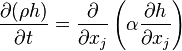\frac{ \partial (\rho h)}{\partial t} = \frac{\partial}{\partial x_j}\left( \alpha \frac{\partial h}{\partial x_j} \right)

(7)

.

$h$ is the specific enthalpy, $\rho$ the density and $\alpha = \kappa / c_p$ is the thermal diffusivity which is defined as the ratio between the thermal conductivity $\kappa$ and the specific heat capacity $c_p$ . Note that $\kappa$ can be also anisotropic.

The source code can be found in solveSolid.H:

 
 
{
    while (pimple.correctNonOrthogonal())
    {
        fvScalarMatrix hEqn
        (
            fvm::ddt(betav*rho, h)
          - (
                thermo.isotropic()
              ? fvm::laplacian(betav*thermo.alpha(), h, "laplacian(alpha,h)")
              : fvm::laplacian(betav*taniAlpha(), h, "laplacian(alpha,h)")
            )
          ==
            fvOptions(rho, h)
        );
 
        hEqn.relax();
 
        fvOptions.constrain(hEqn);
 
        hEqn.solve(mesh.solver(h.select(pimples.finalIter())));
 
        fvOptions.correct(h);
    
 
thermo.correct();
 
Info<< "Min/max T:" << min(thermo.T()).value() << ' '
    << max(thermo.T()).value() << endl;

1.3 Coupling between Fluid and Solid

A good explanation of the coupling between fluid and solid can be found in https://www.cfd-online.com/Forums/openfoam-solving/143571-understanding-temperature-coupling-bcs.html.

At the interface between solid s and fluid f the temperature T for both phases that to be the same:

T_f = T_s

(8)

.

Furthermore the heat flux entering one region at one side of the interphase should be equal to the heat flux leaving the other region on the other side of the domain:

Q_f = -Q_s

(9)

.

If we neglect radiation the above expression can be written as:

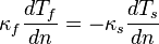\kappa_f \frac{d T_f}{ d n} = - \kappa_s \frac{d T_s}{ d n}

(10)

.

$n$ represents the direction normal to the wall. $\kappa_f$ and $\kappa_s$ are the thermal conductivity of the fluid and solid, respectively.

The source code of the above boundary condition can be found in src/TurbulenceModels/compressible/turbulentFluidThermoModels/derivedFvPatchFields/turbulentTemperatureCoupledBaffleMixed/turbulentTemperatureCoupledBaffleMixedFvPatchScalarField.src/TurbulenceModels/compressible/turbulentFluidThermoModels/derivedFvPatchFields/turbulentTemperatureCoupledBaffleMixed/turbulentTemperatureCoupledBaffleMixedFvPatchScalarField.C

2 Source Code

3 References

↑ EL ABBASSIA, M.; LAHAYE, D. J. P.; VUIK, C. MODELLING TURBULENT COMBUSTION COUPLED WITH CONJUGATE HEAT TRANSFER IN OPENFOAM.

[1] EL ABBASSIA, M.; LAHAYE, D. J. P.; VUIK, C. MODELLING TURBULENT COMBUSTION COUPLED WITH CONJUGATE HEAT TRANSFER IN OPENFOAM.

[1]

@@ Line 363: / Line 363: @@
 </math></center>
 </td><td width="5%">(9)</td></tr></table>.
+If we neglect radiation the above expression can be written as:
+<table width="70%"><tr><td>
+<center><math>
+\kappa_f \frac{d T_f}{ d n} = - \kappa_s \frac{d T_s}{ d n}
+</math></center>
+</td><td width="5%">(10)</td></tr></table>.
+<math> n  </math> represents the direction normal to the wall.  <math> \kappa_f  </math>
+and
+<math> \kappa_s  </math> are the thermal conductivity of the fluid and solid, respectively.
+The source code of the above boundary condition can be found in
+src/TurbulenceModels/compressible/turbulentFluidThermoModels/derivedFvPatchFields/turbulentTemperatureCoupledBaffleMixed/turbulentTemperatureCoupledBaffleMixedFvPatchScalarField.src/TurbulenceModels/compressible/turbulentFluidThermoModels/derivedFvPatchFields/turbulentTemperatureCoupledBaffleMixed/turbulentTemperatureCoupledBaffleMixedFvPatchScalarField.C
 ==Source Code==

Difference between revisions of "ChtMultiRegionFoam"