FireFoam

fireFoam

   Transient solver for fires and turbulent diffusion flames with reacting
   particle clouds, surface film and pyrolysis modelling.

1 Solution Strategy

The source code can be found in fireFoam.C

 
 
/*---------------------------------------------------------------------------*\
  =========                 |
  \\      /  F ield         | OpenFOAM: The Open Source CFD Toolbox
   \\    /   O peration     |
    \\  /    A nd           | Copyright (C) 2011-2017 OpenFOAM Foundation
     \\/     M anipulation  |
-------------------------------------------------------------------------------
License
    This file is part of OpenFOAM.
 
    OpenFOAM is free software: you can redistribute it and/or modify it
    under the terms of the GNU General Public License as published by
    the Free Software Foundation, either version 3 of the License, or
    (at your option) any later version.
 
    OpenFOAM is distributed in the hope that it will be useful, but WITHOUT
    ANY WARRANTY; without even the implied warranty of MERCHANTABILITY or
    FITNESS FOR A PARTICULAR PURPOSE.  See the GNU General Public License
    for more details.
 
    You should have received a copy of the GNU General Public License
    along with OpenFOAM.  If not, see <http://www.gnu.org/licenses/>.
 
Application
    fireFoam
 
Group
    grpCombustionSolvers
 
Description
    Transient solver for fires and turbulent diffusion flames with reacting
    particle clouds, surface film and pyrolysis modelling.
 
\*---------------------------------------------------------------------------*/
 
#include "fvCFD.H"
#include "turbulentFluidThermoModel.H"
#include "basicReactingCloud.H"
#include "surfaceFilmModel.H"
#include "pyrolysisModelCollection.H"
#include "radiationModel.H"
#include "SLGThermo.H"
#include "solidChemistryModel.H"
#include "psiReactionThermo.H"
#include "CombustionModel.H"
#include "pimpleControl.H"
#include "fvOptions.H"
 
// * * * * * * * * * * * * * * * * * * * * * * * * * * * * * * * * * * * * * //
 
int main(int argc, char *argv[])
{
    argList::addNote
    (
        "Transient solver for fires and turbulent diffusion flames"
        " with reacting particle clouds, surface film and pyrolysis modelling."
    );
 
    #include "postProcess.H"
 
    #include "addCheckCaseOptions.H"
    #include "setRootCaseLists.H"
    #include "createTime.H"
    #include "createMesh.H"
    #include "createControl.H"
    #include "createFields.H"
    #include "createFieldRefs.H"
    #include "initContinuityErrs.H"
    #include "createTimeControls.H"
    #include "compressibleCourantNo.H"
    #include "setInitialDeltaT.H"
    #include "createRegionControls.H"
 
    turbulence->validate();
 
    // * * * * * * * * * * * * * * * * * * * * * * * * * * * * * * * * * * * //
 
    Info<< "\nStarting time loop\n" << endl;
 
    while (runTime.run())
    {
        #include "readTimeControls.H"
        #include "compressibleCourantNo.H"
        #include "solidRegionDiffusionNo.H"
        #include "setMultiRegionDeltaT.H"
        #include "setDeltaT.H"
 
        ++runTime;
 
        Info<< "Time = " << runTime.timeName() << nl << endl;
 
        parcels.evolve();
 
        surfaceFilm.evolve();
 
        if(solvePyrolysisRegion)
        {
            pyrolysis.evolve();
        }
 
        if (solvePrimaryRegion)
        {
            #include "rhoEqn.H"
 
            // --- PIMPLE loop
            while (pimple.loop())
            {
                #include "UEqn.H"
                #include "YEEqn.H"
 
                // --- Pressure corrector loop
                while (pimple.correct())
                {
                    #include "pEqn.H"
                }
 
                if (pimple.turbCorr())
                {
                    turbulence->correct();
                }
            }
 
            rho = thermo.rho();
        }
 
        runTime.write();
 
        runTime.printExecutionTime(Info);
    }
 
    Info<< "End" << endl;
 
    return 0;
}
 
 
// ************************************************************************* //
 

2 Equations

2.1 Equations Liquid Film

The equation describing the evolution of the liquid film can be found in http://www.ilasseurope.org/ICLASS/iclass2012_Heidelberg/Contributions/Paper-pdfs/Contribution1294_b.pdf and https://www.witpress.com/Secure/elibrary/papers/MPF11/MPF11020FU1.pdf. A description of the method used to derive the equation can be found in https://www.researchgate.net/profile/Petr_Vita/publication/313655371_Thin_Film_Fluid_Flow_Simulation_on_Rotating_Discs/links/58a1a592a6fdccf5e9707665/Thin-Film-Fluid-Flow-Simulation-on-Rotating-Discs.pdf.

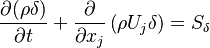
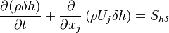
The conservation of mass reads:

$\frac{ \partial (\rho \delta )}{\partial t} + \frac{\partial}{\partial x_j} \left( \rho {U}_{j} \delta \right) = S_{\delta}$

(1)

$U$ represents the mean film velocity, $\delta$ the film height and $S_\delta$ mass source term resulting from the impingement of the liquid droplets on the film surface. The source code of the continuity equation can be found in src/regionModels/surfaceFilmModels/kinematicSingleLayer:

 
void kinematicSingleLayer::solveContinuity()
{
    if (debug)
    {
        InfoInFunction << endl;
    }
 
    solve
    (
        fvm::ddt(deltaRho_)
      + fvc::div(phi_)
     ==
      - rhoSp_
    );
}

The momentum conservation reads:

$\frac{ \partial (\rho \delta U)}{\partial t} + \frac{\partial}{\partial x_j} \left( \rho U_i {U}_{j} \delta \right) = -\delta \frac{\partial p}{\partial x_i} + \tau + S_{U\delta}$

(2)

$p$ represents the pressure, $\tau$ the stress like components of the forces acting on the filme and $S_{U\delta}$ represents the contribution to the momentum by the impinging droplets. The pressure contribution is divided in three components: The contribution due to capillary effects 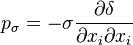$p_\sigma = -\sigma\frac{\partial \delta }{\partial x_i \partial x_i}$, the hydrostatic contribution 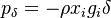$p_\delta = - \rho x_i g_i \delta$ and the contribution of the pressure originated by the surrounding gas $p_g$ . $\sigma$ represents the surface tension. The stress like contribution is divided in the wall shear stress 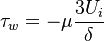$\tau_w =- \mu \frac{ 3 U_i}{\delta}$ , the gravity force tangential to the wall $\tau_t = \rho \delta g_{ti}$ and the contribution of the contact line force $\tau_\theta$. $g_{ti}$ is the component of the gravity parallel to the wall. Finally the momentum equation can be written as:

$\frac{ \partial (\rho \delta U)}{\partial t} + \frac{\partial}{\partial x_j} \left( \rho U_i {U}_{j} \delta \right) = -\delta \frac{\partial}{\partial x_i} \left ( - \rho x_i g_i \delta -\sigma\frac{\partial \delta }{\partial x_i \partial x_i} + p_g \right ) + \rho \delta g_{ti} - \mu \frac{ 3 U_i}{\delta} + \tau_\theta + S_{U\delta}$

(3)

The source code of the momentum equation can be found in src/regionModels/surfaceFilmModels/kinematicSingleLayer:

 
tmp<Foam::fvVectorMatrix> kinematicSingleLayer::solveMomentum
(
    const volScalarField& pu,
    const volScalarField& pp
)
{
    if (debug)
    {
        InfoInFunction << endl;
    }
 
    // Momentum
    tmp<fvVectorMatrix> tUEqn
    (
        fvm::ddt(deltaRho_, U_)
      + fvm::div(phi_, U_)
     ==
      - USp_
   // - fvm::SuSp(rhoSp_, U_)
      - rhoSp_*U_
      + forces_.correct(U_)
      + turbulence_->Su(U_)
    );
 
    fvVectorMatrix& UEqn = tUEqn.ref();
 
    UEqn.relax();
 
    if (momentumPredictor_)
    {
        solve
        (
            UEqn
         ==
            fvc::reconstruct
            (
              - fvc::interpolate(delta_)
              * (
                    regionMesh().magSf()
                  * (
                        fvc::snGrad(pu, "snGrad(p)")
                      + fvc::snGrad(pp, "snGrad(p)")*fvc::interpolate(delta_)
                      + fvc::snGrad(delta_)*fvc::interpolate(pp)
                    )
                  - fvc::flux(rho_*gTan())
                )
            )
        );
 
        // Remove any patch-normal components of velocity
        U_ -= nHat()*(nHat() & U_);
        U_.correctBoundaryConditions();
    }
 
    return tUEqn;
}

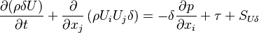
The energy equation reads:

$\frac{ \partial (\rho \delta h )}{\partial t} + \frac{\partial}{\partial x_j} \left( \rho {U}_{j} \delta h \right) = S_{h\delta}$

(4)

$h$ represents the mean film enthalpy and $S_{h\delta}$ represents the contribution of the impinging droplets to the energy equation. The source code can be found in src/regionModels/surfaceFilmModels/thermoSingleLayer:

 
void thermoSingleLayer::solveEnergy()
{
    if (debug)
    {
        InfoInFunction << endl;
    }
 
 
    dimensionedScalar residualDeltaRho
    (
        "residualDeltaRho",
        deltaRho_.dimensions(),
        1e-10
    );
 
    solve
    (
        fvm::ddt(deltaRho_, hs_)
      + fvm::div(phi_, hs_)
     ==
      - hsSp_
      + q(hs_)
      + radiation_->Shs()
    );
 
    correctThermoFields();
 
    // Evaluate viscosity from user-model
    viscosity_->correct(pPrimary_, T_);
 
    // Update film wall and surface temperatures
    updateSurfaceTemperatures();
}

Equations (1), (3) and (4) represent a system of 3 non-linear partial differential equations with the unknowns $\delta$, $U_i$ and $h$. In order to solve this system of equations, a splitting method is adopted: The equations are linearised by using quantities from the previous iteration and solved sequentially. The steps performed are the following:

1. Solve continuity equation (1). Here has to be mentioned that the quantity solved for is $\rho_\delta = \rho \delta$ which appears also in the momentum and energy equation.

2. Solve momentum equation (3)

3. Solve energy equation (4)

4. Solve film thickness equation: The film thickness equation is derived by inserting the discrete momentum equation into the continuity equation.

Steps 2-4 are solved a number of time specified by the user in order to achieve sufficient convergence of the equations. The source code can be found in src/regionModels/surfaceFilmModels/thermoSingleLayer

 
 
 void thermoSingleLayer::evolveRegion()
{
    if (debug)
    {
        InfoInFunction << endl;
    }
 
    // Solve continuity for deltaRho_
    solveContinuity();
 
    // Update sub-models to provide updated source contributions
    updateSubmodels();
 
    // Solve continuity for deltaRho_
    solveContinuity();
 
    for (int oCorr=1; oCorr<=nOuterCorr_; oCorr++)
    {
        // Explicit pressure source contribution
        tmp<volScalarField> tpu(this->pu());
 
        // Implicit pressure source coefficient
        tmp<volScalarField> tpp(this->pp());
 
        // Solve for momentum for U_
        tmp<fvVectorMatrix> UEqn = solveMomentum(tpu(), tpp());
 
        // Solve energy for hs_ - also updates thermo
        solveEnergy();
 
        // Film thickness correction loop
        for (int corr=1; corr<=nCorr_; corr++)
        {
            // Solve thickness for delta_
            solveThickness(tpu(), tpp(), UEqn());
        }
    }
 
    // Update deltaRho_ with new delta_
    deltaRho_ == delta_*rho_;
 
    // Update temperature using latest hs_
    T_ == T(hs_);
}
 

2.2 Equations Fluid

2.2.1 Momentum conservation

The equation of motion are written for a moving frame of reference. They are however formulated for the absolute velocity (the derivation of the equations of motion can be found in https://openfoamwiki.net/index.php/See_the_MRF_development and also in https://diglib.tugraz.at/download.php?id=581303c7c91f9&location=browse. Some additional information can be found in https://pingpong.chalmers.se/public/pp/public_courses/course07056/published/1497955220499/resourceId/3711490/content/UploadedResources/HakanNilssonRotatingMachineryTrainingOFW11-1.pdf):

$\frac{ \partial (\rho {u}_i)}{\partial t} + \frac{\partial}{\partial x_j} \left( \rho {u}_{rj} u_i \right) + \rho\epsilon_{ijk}\omega_i u_j= - \frac{\partial p_{rgh}} {\partial{x_i}} - \frac{\partial \rho g_j x_j}{\partial x_i} + \frac{\partial}{\partial x_j} \left( \tau_{ij} + \tau_{t_{ij}} \right) + F_{pi}$

(2)

$u$ represent the velocity, $u_r$ the relative veloicty, $g_i$ the gravitational acceleration, 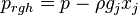$p_{rgh} = p - \rho g_j x_j$ the pressure minus the hydrostatic pressure and $\tau_{ij}$ and $\tau_{t_{ij}}$ are the viscose and turbulent stresses. Note that since the relative velocity $u_r$ appears in the divergence term, the face flux $\phi$ appearing in the finite volume discretization of the momentum equation should be calculated with the relative velocity. $F_{pi}$ represents the force excreted by the particles on the fluid.

The source code can be found in Ueqn.H:

 
 
      MRF.correctBoundaryVelocity(U);
 
    fvVectorMatrix UEqn
    (
        fvm::ddt(rho, U) + fvm::div(phi, U)
      + MRF.DDt(rho, U)
      + turbulence->divDevRhoReff(U)
     ==
        parcels.SU(U)
      + fvOptions(rho, U)
    );
 
    UEqn.relax();
 
    fvOptions.constrain(UEqn);
 
    if (pimple.momentumPredictor())
    {
        solve
        (
            UEqn
          ==
            fvc::reconstruct
            (
                (
                  - ghf*fvc::snGrad(rho)
                  - fvc::snGrad(p_rgh)
                )*mesh.magSf()
            )
        );
 
        fvOptions.correct(U);
        K = 0.5*magSqr(U);
    }