OpenFOAM guide/The PIMPLE algorithm in OpenFOAM

1 Storyboard

First I wanted to write a nice story like »Ignaz« but that would only copy the good attention of the author and of course I am not a good story-teller. Therefor I will go directly to the topic and will tell you how the PIMPLE algorithm is working in OpenFOAM, how to set up the keywords and which abilities you have to control the algorithm. The test case it the pitzDaily case in the pimpleFoam folder of incompressible fluids. Only the courant number was decreased to 3.

2 Case A

In the first case we are using the tutorial case and change the fvSolution file. In the pimple control directory we will remove all entrys to get only a dummy body.

 
PIMPLE
{
}

After starting the simulation you can see that the solver is still running but after a while it will crash. The following questions occur at that case:

1. why is the solver working without complaining that keywords are missing
2. in which mode is the solver running when there are no keywords

Question 1:

If you don't insert any keywords into the PIMPLE control dictionary, the solver is still running using the default settings. After calling the pimpleControl the solver initialize the necessary keywords with default values. These can be cecked out in the pimpleControl.C file:

 
   121 // * * * * * * * * * * * * * * * * Constructors  * * * * * * * * * * * * * * // 
   122 
   123 Foam::pimpleControl::pimpleControl(fvMesh& mesh)
   124 :
   125     solutionControl(mesh, "PIMPLE"),
   126     nCorrPIMPLE_(0),
   127     nCorrPISO_(0),
   128     corrPISO_(0),
   129     turbOnFinalIterOnly_(true),
   130     converged_(false)
   131 {   
   132     read();

As you can see there are several keywords that can be used if you are using the PIMPLE algorithm. These keywords are set »by default« to the values you can see at the code above. After initialize the values, the constructor will call the »read()« function which will check out the user defined values and overwrite the above values with user values or other values which are necessary that the solver is working. If there are no values in the PIMPLE control available the solver is using the default one. The functions is given below:

 
    39 void Foam::pimpleControl::read()    
    40 {
    41     solutionControl::read(false);
    42 
    43     // Read solution controls
    44     const dictionary& pimpleDict = dict();
    45     nCorrPIMPLE_ = pimpleDict.lookupOrDefault<label> ("nOuterCorrectors", 1);
    46     nCorrPISO_ = pimpleDict.lookupOrDefault<label>("nCorrectors", 1);
    47     turbOnFinalIterOnly_ =
    48         pimpleDict.lookupOrDefault<Switch>("turbOnFinalIterOnly", true);
    49 }

As you can see here, this function is looking in the fvSolution file for some entrys in the PIMPLE control structure:

nOuterCorrctors (nCorrPIMPLE) is set by default to 1
nCorrectors (nCorrPISO) is set by default to 1
nNonOrthogonalCorrectors (corrPISO) is set by default to 0  (not shown here)
turbOnFinalIterOnly is set by default to true
Residual control is  set to false

Question 2:

If you are running the PIMPLE solver without any keywords it is operating in PISO mode and therefor you need very small time steps. Thats the reason why the simulation will blow up with these settings (Co = 3). That the solver is operating in PISO mode can be shown in the source code too, and will report it on the screen:

 
  134     if (nCorrPIMPLE_ > 1)   
  135     {
   .
   .
   .
   156     }
   157     else
   158     {
   159         Info<< nl << algorithmName_ << ": Operating solver in PISO mode" << nl
   160             << endl;
   161     }

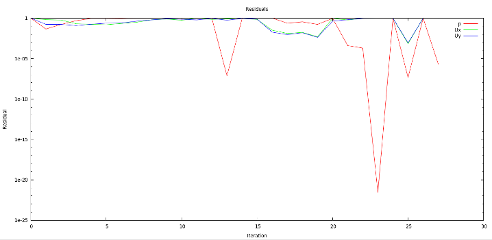
Residuals if you are using a empty PIMPLE directory

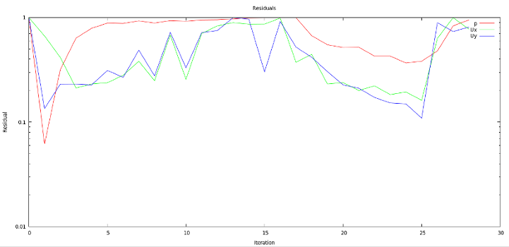
As you can see the residuals are not converging and the solution blow up. The reason is due to the high Co number (Co = 3) and the fact that without keywords the PIMPLE algorithm is working in PISO mode. To solve the problem you have to reduce the Co number but that is not is not the aim to introduce merged PISO - SIMPLE algorithm.

Legend:

• Iteration at the bottom means one PISO iteration; that means in each iteration you go on with the time. In other words every iteration solves a new time step.

3 Case B

In the second case we are using the standard entrys in the fvSolution file used in the tutorial.

 
PIMPLE
{
    nCorrectors         2;
}

Now we correct the pressure field twice and that means that we calculate the following equation twice:

$\nabla^2 p = f(U, \nabla p)$

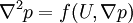
In that case the pressure - momentum coupling is stable enough to work and the solver will not blow up.

Advantage

• While you are using nCorrectors with a number higher than 1 the PIMPLE algorithm is still working in PISO mode with the advantage that you calculate your pressure twice, this is also available in the normal PISO solver but is still not the aim of the PIMPLE solver.

Residuals if you are using the PIMPLE algorithm with nCorrectors 2

The residual of the pressure is much better and the solution is stable in that moment - not tested what happen if you solve more seconds.

Legend:

• For the momentum one iteration means »one time step«, in other words that means in that case we were solving round about 65 time steps
• For the pressure we solve the equation given above two times and therefor it is not anymore possible to say that one iteration is one time step. In that case two iterations are necessary to go on in time.

4 Case C

Now we will use the MERGED PISO - SIMPLE algorithm and therefor we are using the advantage of the SIMPLE mode idea (relaxation). What does that mean? In fact it is really easy. If you are using the PISO mode you are strict limited to the time step (Co < 1). That mean that it is very expensive to solve a real time problem in transient manner for long time especially in very complex geometries. SIMPLE is developed for steady-state condition to reach that state very fast but (normally) does not contain time derivation and therefor no time information. To provide a stable simulation you have to introduce relaxation factors that limit the values of the new values.

$\phi^n = \phi^{n-1} + \alpha_\phi ( \phi^{\mathrm{new}} - \phi^{n-1})$

In other words, the new value $\phi^n$ is a combination of the old value $\phi^{n-1}$ and the new one $\phi^{\mathrm{new}}$ which is calculated. This make the simulation stable but not time conservative. It allows you to reach the steady-state condition very fast; time information is not needed.

Miss understanding

A lot of people miss understand the function of the PIMPLE algorithm. The problem in the case we are using here is, that this case is very simple. Imagine a very complex simulation in which it is very straight forward to simulate small time steps. If you want to have bigger time steps you have to increase your Co number which leads you to unstable convergence. At that moment you are in a discrepancy because you want go on faster in time step to reduce computational effort but it is not possible because you are limited in time step due to the Co number.

4.1 Case C.1

Now we will use the following fvSolution file:

 
PIMPLE
{
    nCorrectors                1;
    nOuterCorrectors    2;
}

Compared to Case B there is not a big difference. The only difference is that we calculate the pressure - momentum coupling in one time step twice:

1. Calculate momentum
2. Calculate pressure
3. Recalculate momentum from new pressure
4. Recalculate pressure from new momentum

1. $\frac{U}{\partial t} + \nabla \cdot (UU) + \nabla \cdot R = -\nabla p$

2. $\nabla^2 p = f(U, \nabla p)$

$\rightarrow p_{\mathrm{new}}$

$\rightarrow$ correct U with $p_{\mathrm{new}} \rightarrow U_\mathrm{corrected}$

$\rightarrow$ now you use the $U_\mathrm{corrected}$ and $p_{\mathrm{new}}$ for the second loop

3. $\frac{U}{\partial t} + \nabla \cdot (UU) + \nabla \cdot R = -\nabla p$

4. $\nabla^2 p = f(U, \nabla p)$

$\rightarrow p_{\mathrm{new}}$

$\rightarrow$ correct U with $p_{\mathrm{new}} \rightarrow U_\mathrm{corrected}$

During this calculation it has not a big advantage and is like Case A calculated twice and then move on in time step (with the only difference, that the turbulence is calculated at the end. That means in PIMPLE Iteration 2 due to the fact that turbOnFinalIterOnly = true). You can assume that the calculation will blow up which is shown in the residual plot.

Residuals if you are using the PIMPLE algorithm with the settings above

As you can see it is much worse compared to Case 1. At that moment there is none advantage of the pimple mode that we are using but we are using it in a wrong way.

4.2 Case C.2

Now we want to generate a complete PIMPLE case. The fvSolution file looks like that:

 
PIMPLE
{
    nNonOrthogonalCorrectors 0;
    nCorrectors          1;
    nOuterCorrectors    2;  // Set to 50 
 
 
relaxationFactors
{
    fields
    {
        p      0.3;
        pFinal   1;
    }
    equations
    {
        "U|k|epsilon"     0.3;
        "(U|k|epsilon)Final"   1;
    }
}

We introduced the relaxation factors to obtain a smooth convergence. The problem now is that we use the relaxation factors in the first pimple loop but after we reach the last one (here iteration 2 because nOuterCorrectors = 2) the relaxation factor will be 1 again to ensure time consistence but this makes no sense in the following case. Therefor we will change the nOuterCorrectors to 50. Now we calculate 50 times the pressure - momentum coupling. Therefor 49 times with relaxation (like SIMPLE) and the last time without relaxation. For cases that are very instable this is perfect to get a smooth convergence. In other words we are using the idea of SIMPLE mode (under relaxation) between the time steps to converge the solution at these time step to a certain limit. The limit is set in a way to be sure the solution is accurate in time and space.

Residuals if you are using the right PIMPLE algorithm with relaxation

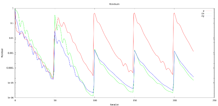
You can see that the solution is stable and the convergence is very good. Further more you can see the pimple loops; here from zero to fifty iteration, 100 to 150 and so on. After you finished the pimple loop we go on in time and do the same thing again. If you introduce the nCorrectors > 1 you will calculate the pressure field n times (more hints to that later).

Do not forget

At the moment we have 50 Iterations per time step and therefor the computational effort could be bigger as befor. To avoid that you should always add residual controls to stop the pimple loop after reaching some special criterion » Case C.3

4.3 Case C.3

At least we introduce the residual control to exit the pimple loop after we reached a good solution during one time step. The fvSolution file looks like that:

 
PIMPLE
{
    nNonOrthogonalCorrectors 0;
    nCorrectors          1;
    nOuterCorrectors    50;
 
    residualControl
    {
        U
        {
                tolerance  1e-5;
                relTol      0;
        }
        p
        {
                tolerance  5e-4;
                relTol      0;
        }
     }
}
 
relaxationFactors
{
    fields
    {
        p      0.3;
        pFinal   1;
    }
    equations
    {
        "U|k|epsilon"     0.3;
        "(U|k|epsilon)Final"   1;
    }
}

Residuals if you are using the right PIMPLE algorithm with relaxation and residualControl

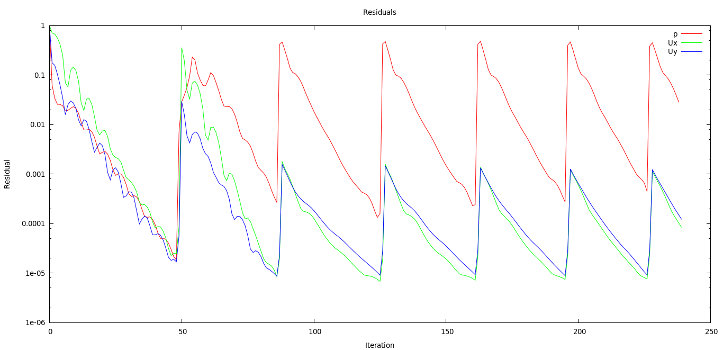
As you can see now, the time iteration is faster because after the pimple loop will reach the residual control it will go to the next time step.

smoothSolver:  Solving for Ux, Initial residual = 2.07804e-06, Final residual = 2.07804e-06, No Iterations 0
smoothSolver:  Solving for Uy, Initial residual = 3.42321e-06, Final residual = 3.42321e-06, No Iterations 0
GAMG:  Solving for p, Initial residual = 0.000407312, Final residual = 3.14679e-08, No Iterations 8
time step continuity errors : sum local = 5.66964e-12, global = 3.09312e-13, cumulative = -8.61807e-06
smoothSolver:  Solving for epsilon, Initial residual = 0.00512886, Final residual = 2.08382e-06, No Iterations 2
smoothSolver:  Solving for k, Initial residual = 0.0660137, Final residual = 1.08191e-06, No Iterations 3
'''PIMPLE: converged in 28 iterations'''
ExecutionTime = 13.84 s  ClockTime = 14 s

Althoug we set 50 iterations for the pimple loop it will exit the loop after the residual control settings are true. That saves computational effort.

5 Some hints

• the pitzDaily tutorial is to easy to show the advantage of PIMPLE in a good manner

• PIMPLE is very effective in big cases to increase the Co number

• PIMPLE speed up your simulation and could reach a stable solution due to under relaxation

• For high turbulent flow you should add turbOnFinalIterOnly = false to your PIMPLE control

• Set nOuterCorrectors up to a very high number (~ 50 to 200) and control your pimple loop with the residual control

• Set nCorrectors to a small number (1 to 3; you have to play around)

• If you set nCorrectors higher it could be possible to leave the pimple loop earlier and prevent extra calculation but could also do the opposite

• nNonOrthogonalCorr means that you correct the pressure field more often with the new calculated one:

$\nabla^2 p = f(U, \nabla p) \rightarrow p_{\mathrm{new}} \rightarrow \nabla^2 p_{\mathrm{new}} = f(U, \nabla p_{\mathrm{new}} ) \rightarrow$ till nNonOrtogonalCorr is reached

• The optimum relaxation factors depend on the simulation case you are running
• The converged solution is independed of the relaxation factors which are applied
• Due to the fact that you have bigger time steps it could happen that some phsics are not resolved (extrem fast pressure drop etc.)
• At the beginning of an transient simulation it could happen that after 100 pimple loops the solution is still not converged but this will change during the simulation time

• simple heat transfer case has at the beginning 200 pimple loops and is still not converging
• after the tenth time step it converges and the pimple loops decrease significantly till it get a steady state pimple iteration of round about 3 - 5

Please feel free to change this site if I got something wrong