Sig Turbomachinery / ERCOFTAC centrifugal pump with a vaned diffuser
Contents
- 1 Testcase description and experimental results
- 2 Published computational results
- 3 References
- 4 Geometric data of the ERCOFTAC centrifugal pump [2][3][4]
- 5 How to get the files
- 6 Directory structure
- 7 Test cases
- 8 Optional tools
- 9 Howtos
- 10 Others
1 Testcase description and experimental results
Olivier Petit, Chalmers University of Technology, Gothenburg, Sweden
Maryse Page, Hydro-Québec, Varennes, Canada
Håkan Nilsson, Chalmers University of Technology, Gothenburg, Sweden
Martin Beaudoin, Hydro-Québec, Varennes, Canada
The testcase was presented by Combès [1] at a Turbomachinery Flow Prediction ERCOFTAC Workshop. The simplified model of the centrifugal pump has 7 impeller blades, 12 diffuser vanes and 6% vaneless radial gap. More information about the geometry and the operating conditions are described in the paper of Ubaldi, Zunino, Barigozzi and Cattenei [2]. The geometry is illustrated in Figure 1.

Figure 1: Impeller and vaned diffuser geometry (Image taken from Ubaldi, Zunino, Barigozzi and Cattanei [2])
The experimental data was provided by Ubaldi et al. [2][3][4]. The model operates in an open circuit with air directly discharged into the atmosphere from the radial diffuser. The pump operates at the nominal operating condition, at a constant rotational speed of 2000 rpm. (Reynolds number: 6.5x10^5, incompressible flow regime). Phase locked ensemble averaged velocity components have been measured with hot wire probes at the impeller outlet. The data includes the distribution of the ensemble averaged static pressure at the impeller front end, taken by means of miniature fast response transducers mounted at the stationary casing of the impeller. LDV measurements were also performed in the impeller and in the diffuser.
It is interesting to note that two-component LDV measurements of the vane unsteady boundary layer were recently published by Canepa, Cattanei, Ubaldi and Zunino [5]. Also, detailed flow measurements within the impeller and the vaneless diffuser have also been published [6]. It is the same impeller used in the measurements of the pump [2][3][4].
2 Published computational results
Computations have been performed by Bert, Combès and Kueny [7][8][9], Torbergsen and White [10], Sato and He [11][12][13], and Théroux et al [14][15]. A 2D model corresponding to a meridional plane with a radial inlet, and a 3D model were initially analyzed by Bert. His work showed that relevant information could be recovered from 2D simulations although the real flow has 3D features. Torbergsen also made computations with a 2D model. Sato and He performed a 3D simulation of a single impeller and two (2/14 instead of 2/12) diffuser blade passages, and a complete 3D model. Théroux analyzed two unsteady 2D models: complete (7 rotors/12 stators) and simplified (1 rotor/2 stators). The simplified 2D model yielded pressure fluctuations caused by rotor-stator interactions that were comparable to those of the complete 2D model.
Preliminary results have shown that OpenFOAM can produce similar results as other CFD codes for frozen rotor computations [16].
Future publications that use this validation test case should refer to Petit et al. [17] and [19].
A thorough study of different numerical settings was done by Xie [18].
3 References
[1] Combès, J.F., "Test Case U3: Centrifugal Pump with a Vaned Diffuser", ERCOFTAC Seminar and Workshop on Turbomachinery Flow Prediction VII, Aussois, jan 4-7 , 1999.
[2] Ubaldi, M., Zunino, P., Barigozzi, G. and Cattanei, A., "An Experimental Investigation of Stator Induced Unsteadiness on Centrifugal Impeller Outflow", Journal of Turbomachinery, vol.118, 41-54, 1996.
[3] Ubaldi, M., Zunino, P., Barigozzi, G. and Cattanei, A., "LDV Investigation of the Rotor-Stator Aerodynamic Interaction in a Centrifugal Turbomachine", 8th International Symposium on Applications of Laser Techniques to Fluid Mechanics, Lisbon, 1996.
[4] Ubaldi, M., Zunino, P. and Cattanei, A., "Etude expérimentale de l'écoulement instationnaire dans le diffuseur aubé d'une turbomachine centrifuge", La Houille Blanche, no 3/4, 31-37, 1998.
[5] Canepa, E., Cattenei, A., Ubaldi, M. and Zunino, P., "Wake-boundary layer interaction on the vaned diffuser of a centrifugal state", Proc. IMechE, vol. 219, Part A: J. Power and Energy, 401-411, 2005.
[6] Ubaldi, M., Zunino, P. and Ghiglione, A., "Detailed flow measurements within the impeller and the vaneless diffuser of a centrifugal turbomachine", Exp. Thermal and Fluid Sci., vol.17, 147-155, 1998.
[7] Bert, P.F., "Modélisation des écoulements instationnaires dans les turbomachines par une méthode éléments finis", Doctoral Thesis, Institut National Polytechnique de Grenoble, 1996.
[8] Bert, P.F., Combès, J.F. and Kueny, J.L., "Unsteady Flow Calculation in a Centrifugal Pump Using a Finite Element Method", Proceedings of the XVIII IAHR Symposium on Hydraulic Machinery and Cavitation, 371-380, 1996.
[9] Combès, J.F., Bert, P.F. and Kueny, J.L., "Numerical Investigation of the Rotor-Stator Interaction in a Centrifugal Pump Using a Finite Element Method", Proceedings of the 1997 ASME Fluids Engineering Division Summer Meeting, FEDSM97-3454, 1997.
[10] Torbergsen, E. and White, M.F., "Transient Simulation of Impeller/Diffuser Interactions", Proceedings of the 1997 ASME Fluids Eng Division Summer Meeting, FEDSM97-3453, 1997.
[11] Sato, K., "Blade Row Interaction in Radial Turbomachines", Ph.D. Thesis, Durham University, 1999.
[12] He, L. and Sato, K., "Numerical Solution of Incompressible Unsteady Flows in Turbomachinery", Proceedings of the 3rd ASME/JSME Joint Fluids Eng Conf, FEDSM99-6871, San Francisco, 1999.
[13] Sato, K. and He, L. "Numerical investigation into the effects of a radial gap on hydraulic turbine performance", Proc. Instn Mech Engrs, vol. 215 Part A, 99-107, 2001.
[14] Théroux, E., "Modélisation numérique des écoulements instationnaires dans les turbomachines radiales", Master Thesis, École Polytechnique de Montréal, 2003.
[15] Page, M., Théroux, E. and Trépanier, J.-Y., "Unsteady rotor-stator analysis of a Francis turbine", 22nd IAHR Symposium on Hydraulic Machinery and Systems, June 29 – July 2, 2004 Stockholm - Sweden.
[16] Page, M. and Beaudoin, M., "Adapting OpenFOAM for Turbomachinery Applications", Second OpenFOAM Workshop, Zagreb, 7-9 June 2007 (slides)
[17] Petit, P., Page, M., Beaudoin, M., Nilsson, H., "The ERCOFTAC centrifugal pump OpenFOAM case-study", 3rd IAHR International Meeting of the Workgroup on Cavitation and Dynamic Problems in Hydraulic Machinery and Systems, October 14-16, 2009, Brno, Czech Republic (paper, poster)
[18] Xie, S., "Studies of the ERCOFTAC Centrifugal Pump with OpenFOAM", Master's Thesis 2010:13, Chalmers University of Technology, ISSN 1652-8557, report
[19] Petit, P. and Nilsson, H. "Numerical Investigations of Unsteady Flow in a Centrifugal Pump with a Vaned Diffuser", International Journal of Rotating Machinery, Volume 2013 (2013), Article ID 961580, 14 pages, http://dx.doi.org/10.1155/2013/961580
4 Geometric data of the ERCOFTAC centrifugal pump [2][3][4]
The case is set up according to the instructions in the ERCOFTAC database. The different parameters used in this case are showed below:
Impeller
Inlet blade diameter 
Outlet diameter 
Number of blades 
Blade span 
Diffuser
Inlet vane diameter 
Outlet vane diameter 
Number of vanes 
Outlet diameter 
Operating conditions
Rotational speed 
Impeller tip speed 
Flow rate coefficient 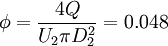
Total pressure rise coefficient 
Reynolds number 
Air density 
The simulated test cases are 2D simulation, so that the blade span of the impeller and the diffuser is not taken into account.
Calculated datas for 2D case
Inlet diameter 
Z thickness 
Flow rate 
Inlet radial speed U0 
5 How to get the files
The OpenFOAM ERCOFTAC Centrifugal Pump cases described in the following sections were developed as a case-study for the Fourth OpenFOAM Workshop, Montréal, 2009, and can be found at the OpenFOAM-extend SourceForge project. It includes complete OpenFOAM cases that solve the flow in the domain (2D) and automatic post-processing of the results. The block-structured hexahedral mesh was generated in ICEM CFD, in two parts - the rotor and the stator. The cases were developed using OpenFOAM-1.5-dev, and some of the features require a recent revision of that release (at this moment, svn version 1238 --Olivierp 16:51, 13 May 2009 (UTC) ). Instructions on how to run the cases follow below.
Get all the current case files by doing:
 cd $FOAM_RUN
 svn checkout svn://svn.code.sf.net/p/openfoam-extend/svn/trunk/Breeder_1.5/OSIG/TurboMachinery/ercoftacCentrifugalPump
In the descriptions below, we thus assume that the ercoftacCentrifugalPump directory is located in the $FOAM_RUN directory
Update your files every now and then by doing:
 cd $FOAM_RUN/ercoftacCentrifugalPump
 svn update
See further info at OpenFOAM-extend webpage
You will also need the profile1DfixedValue boundary condition. To install and use it, see Sig Turbomachinery Library OpenFoamTurbo
6 Directory structure
The structure of the ercoftacCentrifugalPump directory is as follows:
ercoftacCentrifugalPump
 |-- cases
 |-- measurements
- The "cases" directory contains the different test cases.
- The "measurements" directory contains all the data measured by Ubaldi et al. ([1] [2]) in their experimental investigations for the ERCOFTAC testcase. The data is re-arranged to facilitate the automatic post-processing.
Here is what you can find in the "cases" directory:
cases
     |-- MRFSimpleFoam
         |-- ECPGgi2D
         |-- ECPStitchMesh2D
         |-- ECPMixingPlane2D        *
     |-- simpleTurboMFRFoam          *
         |-- ECPGgi2D                *
         |-- ECPStitchMesh2D         *
         |-- ECPMixingPlane2D        *
     |-- turbDyMFoam                 *
         |-- ECPMixerGgiFvMesh2D
         |-- ECPMixerFvMesh2D        *
     |-- meshes

*: Those cases are not yet shared in the svn but it is planned to release them
All cases have the same sub-directory structure. Here is an example based on the MRFSimpleFoam/ECPGgi2D case:
ECPGgi2D
   |-- ECPGgi2D_orig
   |-- rotor2D_orig
   |-- stator2D_orig
   |-- postProcessing
   |-- Allrun
   |-- Allclean
   `-- 00README
- The *_orig files are the original files, and should never be touched. The Allrun and Allclean scripts require that these are the original files checked out from the repository.
- In the "meshes" directory, the Fluent meshes (generated in ICEM CFD) are located. The same meshes are used for several cases, but a single file is used to save disk space.
You can contribute cases if you come up with more ideas. In that case, please try to follow the same directory structure and name conventions. Add instructions on the new cases in this Wiki.
7 Test cases
7.1 MRFSimpleFoam
7.2 simpleTurboMFRFoam
7.3 turbDyMFoam
7.4 transientSimpleDyMFoam
7.5 Descriptions of the scripts used in the cases
7.5.1 The Allrun script
The Allrun script is identical for all the MRFSimpleFoam cases. Here is a short description of the different steps that are executed in this script:
- Do a copy of the initial directories.
- Convert the rotor and stator mesh, written in Fluent format, into OpenFOAM format.
- (optional) If you want to compare the computation with the experimental data, you need to do 4 simulations at 4 different rotor positions, corresponding to the four different positions described in the paper published by Ubaldi et al. [1]. It is possible to do the four simulations one after the other by taking away the comments from one of the three lines in "creating the mesh", thus rotating the rotor mesh to a new position.
- Call out an other script, makeMesh that will differ whether the GGI interface is used or if the different parts of the mesh are stitched.
- Once the makeMesh script is done, the simulation starts.
7.5.2 The makeMesh script used in MRFSimpleFoam/ECPGgi2D
This script is called by Allrun, and builds the ECPGgi2D case. It is divided into 3 steps:
- Merging the mesh, using mergeMeshes
- Setting up the case to make it work with MRFSimpleFoam, that is to say, creating the cell and faceZones that define the rotating part of the mesh
- Setting up the case to make it work with the GGI interface
7.5.3 The makeMesh script used in MRFSimpleFoam/ECPStitchMesh2D
This script is called by Allrun, and builds the ECPStitchMesh2D case. It is divided into 3 steps:
- Merging the two parts of the mesh
- Stitching the two different mesh parts
- Setting up the case to make it work with MRFSimpleFoam
7.5.4 The makeMesh script used in simpleTurboMFRFoam/ECPGgi2D
This script is called by Allrun, and builds the ECPGgi2D case. It is divided into 3 steps:
- Merging the two parts of the mesh
- Stitching the two different mesh parts
- Creating a field alpha of value 0 or 1 that define the rotating part of the mesh, using setFields.
7.5.5 Allrun post-processing
The post-processing automatization consists in three steps:
- Post-processing the data, and calculating the velocity magnitude as well as the velocity components, using foamCalc
- Sampling on the latest time. this will sample the data on a list of points that is given in system/sampleDict, and that corresponds to a circle of radius R = R2 * 1.02, where R2 is the outer radius of the impeller.
- Compare the computational results with the experimental ones using gnuplot, and visualize an html file with help of Mozilla or your favorite web browser.
See further info about:
- mergeMeshes at HowTo: mergeMeshes
- stitchMesh at HowTo: stitchMesh
- The GGI interface at HowTo: GGI interface
- The MRFSimpleFoam solver at HowTo: MRFSimpleFoam
7.6 Check list in case of errors during the simulations
If the simulation doesn't start when using the Allrun scripts, please check that:
- You do have the development version of OpenFOAM 1.5 (OpenFOAM-1.5-dev).
- You have the latest update of the development version, at this moment, svn version 1238 ( --Olivierp 16:53, 13 May 2009 (UTC) ).
- You have compiled the MRFSimpleFOAM that is located in $FOAM_TUTORIALS/MRFSimpleFoam.
- You have compiled the simpleTurboMFRFoam that is located in $FOAM_TUTORIALS/simpleTurboMFRFoam.
- You have compiled the boundary condition turboWallFixedValue.
- You have compiled the boundary condition profile1D velocity, and that you have the profile datafile (*.csv) in constant/.
- You have compiled the simpleFunctionObjects library available from the Breeder_1.5 section of the Subversion repository of the project openfoam-extend on SourceForge.NET. By default this tutorial uses the trackDictionary functionObject from this library. In case you do not want to use it, simply delete or comment the lines relative to the trackDictionary functionObject in system/controlDict.
- For the post-processing, the Web browser mozilla is used to visualize the results. It is possible to use another browser; just modify the visualizing command in Allrun accordingly.
- Check again that all the points listed above are validated.
8 Optional tools
This part shows some tools that can be used to simplify the set-up. Some of those tools were created just after the release of OpenFOAM 1.5-dev and are still evolving. They usually tend to be very useful, and it is recommended to use them.
8.1 The ggiCheck functionObject
The ggiCheck functionObject is already integrated in the OpenFOAM 1.5-dev version, and allows the user to see very easily whether the flux across the GGI interface is balanced or not.
8.1.1 Usage
In order to activate the ggiCheck functionObject, the following set of instructions needs to be written at the end of the case system/controlDict file:
 functions
 (
    ggiCheck
     {

        type ggiCheck;     ## Type of functionObject
        phi phi;           ## parameter that you want to follow through the GGI interface.
                           ## Note that the two parameters have to be the same to have a logical comparison.

        functionObjectLibs ("libsampling.so");  ## Where to load it from (if not already in solver)
     }
  );
8.1.2 Interpretation of the information generated by the ggiCheck functionObject
- During the computation, the ggiCheck functionObject will show this information at each time step:
GGI pair (GGI_INT, GGI_EXT) : 0.00721712 0.00728697 Diff = -1.02048e-06 or 0.0141397 %
This shows the amount of flux going through the GGI patches pair called GGI_INT and GGI_EXT, and the absolute and relative differences between both values.
In that specific example, we can see that the flux unbalance is of the order of 10e-6 or 0.01%.
As a rule of thumb, these difference values should always be very low, and even lower as the computation converges. Otherwise, this might indicate a problem with the GGI interface, or with the mesh topology on each side of the GGI interface.
8.2 The trackDictionary functionObject
During a computation, it is often important to keep a trace of the initial set of parameters that were used to perform it, and also to keep track of any changes made to these parameters. The trackDictionary functionObject was developped for this purpose.
At the start of the computation, the trackDictionary functionObject first writes at the console the value of all the known simulation switches (DebugSwitches, InfoSwitches, OptimisationSwitches, Tolerances, DimensionedConstants). Most of those simulation switches are present in the main controlDict file of any OpenFOAM installation, but some of them are not.
Then the content of a user-supplied list of dictionaries is dumped to the console as well. Some user-defined "begin" and "end" separators are provided in order to easily extract this information back from logfiles when post-processing the case.
If the parameter "runTimeModifiable" is set to "yes" in the case system/controlDict file, then this list of dictionaries will also be checked at every time step in order to detect possible file modifications. If so, the dictionary file content will be dumped to the console again.
8.2.1 Installing the trackDictionary functionObject
This function object is provided by the simpleFunctionObjects library available from the Breeder_1.5-dev section of the Subversion repository from the openfoam-extend project on SourceForge.NET.
The instructions below assume that you have checked-out the library in $WM_PROJECT_USER_DIR:
OpenFOAM-1.5-dev:
cd $WM_PROJECT_USER_DIR
 svn checkout svn://svn.code.sf.net/p/openfoam-extend/svn/trunk/Breeder_1.5/libraries/simpleFunctionObjects/ ./Breeder_1.5/libraries/simpleFunctionObjects/
 cd $WM_PROJECT_USER_DIR/Breeder_1.5/libraries/simpleFunctionObjects/
 wmake libso
OpenFOAM-1.6-ext:
cd $WM_PROJECT_USER_DIR
 svn checkout svn://svn.code.sf.net/p/openfoam-extend/svn/trunk/Breeder_1.6/libraries/simpleFunctionObjects ./Breeder_1.6/libraries/simpleFunctionObjects/
 cd $WM_PROJECT_USER_DIR/Breeder_1.6/libraries/simpleFunctionObjects/
 wmake libso
Note that this will checkout and compile the complete simpleFunctionObjects library, not just the trackDictionary functionObject.
For more information on the simpleFunctionObjects library, please refer to this section of the OpenFOAM Wiki: http://openfoamwiki.net/index.php/Contrib_simpleFunctionObjects
8.2.2 Usage
Once the library is compiled, it is necessary to to activate the trackDictionary functionObject by adding the following instructions at end of the system/controlDict:
    ///////////////////////////////////////////////////////////////////////////////
    // Track the content of a given list of dictionaries for modification
    // throughout a simulation run, and print them to the console when
    // modified.
    //
    // The list of all known switches (DebugSwitches, etc) defined in the
    // main controlDict and by the application and libraries is also echoed
    // at the beginning of the run.
    //
    // It is also possible to specify optional user-defined start and end
    // of section separators in order to facilitate the recovery of the
    // information  at runtime or during the postProcessing of the logged
    // information
    //
    functions
    (
        trackDictionaryContent
        {
            type trackDictionary;

            // Where to load it from (if not already in solver)
            functionObjectLibs ("libsimpleFunctionObjects.so");

            // Names of dictionaries to track.
            dictionaryNameList
            (
                "system/controlDict"
                "system/fvSchemes"
                "system/fvSolution"
                "constant/transportProperties"
                "constant/RASProperties"
            );

             // Boolean flags for enabling/disabling the echo of the
             // main controlDict switches
             echoControlDictDebugSwitches        false;
             echoControlDictInfoSwitches         true;
             echoControlDictOptimisationSwitches true;
             echoControlDictTolerances           true;
             echoControlDictDimensionedConstants true;

             // Section separators (optional)
             // If the string "_sectionIdToken_" explicitely appears in the
             // specification of the following section separators, this token
             // string will be replaced by the name of the dictionary being
             // dumped to the console, plus the file modification date and time.
             sectionStartSeparator "############ Start of: _sectionIdToken_ ############";
             sectionEndSeparator   "############ End of: _sectionIdToken_ ############";
        }
    );
    ///////////////////////////////////////////////////////////////////////////////
In that example, the list of dictionaries is completely user-defined; same with the string values for the section separators named sectionStartSeparator and sectionEndSeparator.
So, for example, if there is a need to track yet another dictionary during a run ( such as constant/MRFZones or constant/dynamicMeshDict), then one only needs to add the file relative pathname to the list dictionaryNameList.
8.3 Enabling non-orthogonal correction for the GGI interface patches
A global switch called enableGgiNonOrthogonalCorrection enables the activation of non-orthogonal correction for the GGI interface patches. This flag is located in the section called OptimisationSwitches in the main controlDict file.
Preliminary tests have shown that enabling non-orthogonal correctors for the GGI interface patches can be required for skewed meshes, namely if the linearUpwind is used as divScheme. It should be noted that this remark is applicable only for schemes which appeal to non-orthogonal correctors. Here is a list schemes using non-orthogonal correction on the boundary patches:
gradSchemes/fourthGrad
gradSchemes/extendedLeastSquaresGrad
gradSchemes/leastSquaresGrad
snGradSchemes/correctedSnGrad
surfaceInterpolation/schemes/skewCorrected
surfaceInterpolation/limitedSchemes/DeferredCorrectionLimitedScheme
surfaceInterpolation/limitedSchemes/LimitedScheme
surfaceInterpolation/limitedSchemes/linearUpwind
8.3.1 Enabling the enableGgiNonOrthogonalCorrection switch in the main controlDict file
When an OpenFOAM computation starts, it will lookup for the global controlDict file in the following places, and in the following order; as soon as one controlDict is found , the values from this dictionary will be used for overriding the global simulation switches.
1: ~/.OpenFOAM/1.5-dev/controlDict                 (user file : version dependant)
2: ~/.OpenFOAM/controlDict                         (user file : version independant)
3: $WM_PROJECT_INST_DIR/site/1.5-dev/controlDict   (site file:  version dependant, where site is simply the string “site”)
4: $WM_PROJECT_INST_DIR/site/controlDict           (site file : version independant, where site is simply the string “site”)
5: $WM_PROJECT_DIR/etc/controlDict                 (default installation file : version independant)
By default, the main controlDict file is located at $WM_PROJECT_DIR/etc/controlDict, and it is usually a good practice to leave this file unchanged. In order to override the OpenFOAM global swtiches values, one should follow these simple steps:
 mkdir ~/.OpenFOAM
 mkdir ~/.OpenFOAM/1.5-dev/
 cp $WM_PROJECT_DIR/etc/controlDict ~/.OpenFOAM/1.5-dev/
The file ~/.OpenFOAM/1.5-dev/controlDict should now be modified in order to enable the enableGgiNonOrthogonalCorrection switch like this in the OptimisationSwitches section:
OptimisationSwitches
{
   fileModificationSkew 10;
   commsType       nonBlocking; //scheduled; //blocking;
   floatTransfer   0;// Floating transfer not realiable
   nProcsSimpleSum 0;
   nSquaredProjection    0;

   enableGgiNonOrthogonalCorrection 1;   ## By default, this flag is set to 0.
}
A debug flag is also available in order to activate some traces at the simulation console when the GGI non-orthogonal corrector is enabled.
The following flag in the DebugSwitches section of the ~/.OpenFOAM/1.5-dev/controlDict should be enabled :
ggi 1;
If this flag is set to 1, then in the log file, the following messages will appear:
--> FOAM Warning :
   From function ggiFvPatch::makeCorrVecs(vectorField& cv)
   in file fvMesh/fvPatches/constraint/ggi/ggiFvPatch.C at line 159
   --  Enabling GGI non-orthogonality correction for patch: GGI_INT
--> FOAM Warning :
   From function ggiFvPatch::makeCorrVecs(vectorField& cv)
   in file fvMesh/fvPatches/constraint/ggi/ggiFvPatch.C at line 159
   --  Enabling GGI non-orthogonality correction for patch: GGI_EXT
8.4 Using PyFoam to monitor your simulations
PyFoam is a suite of Python utilities developped by Bernhard Gshaider. Using this package it is quite easy, among other things, to check the convergence of your simulations. To install PyFoam, please refer to PyFoam utility
Useful command:
pyFoamPlotWatcher.py log_MRF_0
9 Howtos
9.1 2D simulations
OpenFOAM can be run in pure 2D mode by using a mesh with only one cell in one direction. On the two sides of the mesh that are in the 'third direction', the boundary condition type should be set to 'empty'. The checkMesh utility can be used to verify that both sides have the grid points in the same position. If not, it will complain:
***Number of edges not aligned with or perpendicular to non-empty directions: ????
Writing ???? points on non-aligned edges to set nonAlignedEdges
To correct non alignement, flattenMesh can be used. You can view the problematic points using:
foamToVTK -pointSet nonAlignedEdges
and view them in paraview. If they are few, you can edit the points by hand, by using the point labels in constant/polyMesh/sets/nonAlignedEdges and modify their positions in constant/polyMesh/points.
When you run a solver with the 2D mesh, it is also ESSENTIAL that the number of faces in each 'empty' patch is dividable with the number of cells, meaning that the mesh must have all 'empty' faces in the same patch. This is probably not absolutely necessary for the solver, but that is a check done by OpenFOAM in order to determine if the 2D mesh is set up correctly.
In summary, for 2D, you need a mesh that:
- Has only one cell in the third direction
- Has type 'empty' on the patches in the third direction
- Has all 'empty' faces in the same patch, or evenly distributed in two patches
And it is recommended, in order to do a nice simulation, to have:
- Identical grid point distribution on the empty patches
- Perfectly flat empty patches
If all those conditions are filled, then checkMesh should say:
All edges aligned with or perpendicular to non-empty directions.
A 2D mesh can be extruded from a 3D mesh if all the faces on one side of the third direction are in one patch, see info on HowTo extrudeMesh
9.2 extrudeMesh
A mesh can be extruded in a third direction, yielding a new mesh with a number of layers that are similar. This is useful when making a 2D mesh. If all the boundary faces on one of the sides in the 'third direction' are in the same patch (here named 'front'), the commands are as follows:
 cp $FOAM_UTIL/mesh/generation/extrudeMesh/extrudeProperties constant
 sed -i s/"extrudeModel        wedge;"/"//extrudeModel        wedge;"/g constant/extrudeProperties
 sed -i s/"//extrudeModel        linearNormal;"/"extrudeModel        linearNormal;"/g constant/extrudeProperties
 extrudeMesh -sourceRoot <ROOT> -sourceCase <CASE> -sourcePatch front
 extrudeMesh -surface front.sMesh
Then there is some work with new patch names...
9.3 mergeMeshes
This utility takes the meshes from two different cases and merges them into the master case. Note that the two meshes will keep all their original boundary conditions, so they are not automatically coupled. To couple the meshes, use stitchMesh, described below. Here is a description on how to use mergeMeshes:
mergeMeshes . rotor . stator
mergeMeshes reads the system/controlDict of both cases and uses the startTime, so be careful if you have a moving mesh for example. The first case that you specify (rotor in this case) will be the master, and a new time (startTime+deltaT) will be written in which a new polymesh is located. Move it to the correct position (constant/polyMesh), and you have a case with the merged mesh.
NOTE: If you get the error message "Attempt to cast type mergePolyMesh to type fvMesh" you probably have some functionObjects referred to in one or both of the controlDictionaries of your cases. Comment out that part while running mergeMeshes, and you should be fine. Search the Forum for this error message.
Example, that does this for two cavity cases:
 run
 cp -r $FOAM_TUTORIALS/icoFoam/cavity cavity0
 cp -r $FOAM_TUTORIALS/icoFoam/cavity cavity1
 chmod +w -R cavity* #I need this since I copy from protected files
 sed -i s/fixedWalls/leftWall/g cavity0/constant/polyMesh/blockMeshDict
 sed -i s/"(0 4 7 3)"/"(0 4 7 3)\n)\nwall rightWall0\n("/g cavity0/constant/polyMesh/blockMeshDict
 sed -i s/"(2 6 5 1)"/"(2 6 5 1)\n)\nwall lowerWall\n("/g cavity0/constant/polyMesh/blockMeshDict
 sed -i s/fixedWalls/leftWall1/g cavity1/constant/polyMesh/blockMeshDict
 sed -i s/"(0 4 7 3)"/"(0 4 7 3)\n)\nwall rightWall\n("/g cavity1/constant/polyMesh/blockMeshDict
 sed -i s/"(2 6 5 1)"/"(2 6 5 1)\n)\nwall lowerWall\n("/g cavity1/constant/polyMesh/blockMeshDict
 sed -i s/"(20 20 1)"/"(21 21 1)"/g cavity1/constant/polyMesh/blockMeshDict
 blockMesh -case cavity0
 blockMesh -case cavity1
 transformPoints -translate "(0.1 0 0)" -case cavity1
 mergeMeshes . cavity0 . cavity1
 rm -r cavity1
 rm -r cavity0/constant/polyMesh
 mv cavity0/0.005/polyMesh cavity0/constant
 rmdir cavity0/0.005
 sed -i s/fixedWalls/"leftWall\n{\ntype zeroGradient;\n}\n\nleftWall1\n{\ntype zeroGradient;\n}\n\nrightWall\n{\ntype zeroGradient;\n}\n\nrightWall0\n{\ntype zeroGradient;\n}\n\nlowerWall"/g cavity0/0/p
 sed -i s/fixedWalls/"leftWall\n{\ntype fixedValue;\nvalue uniform (0 0 0);\n}\n\nleftWall1\n{\ntype fixedValue;\nvalue uniform (0 0 0);\n}\n\nrightWall\n{\ntype fixedValue;\nvalue uniform (0 0 0);\n}\n\nrightWall0\n{\ntype fixedValue;\nvalue uniform (0 0 0);\n}\n\nlowerWall"/g cavity0/0/U
 icoFoam -case cavity0
 paraFoam -case cavity0
Choose the last time step and color by pressure. You can see that we have two separate volumes where the flow is computed. If we want to couple the meshes we must use stitchMesh. Click on 'Show Patch Names' and 'Apply' to see that we want to stitch patches rightWall0 and leftWall1...
9.4 stitchMesh
stitchMesh couples two uncoupled parts of the mesh that belong to the same case. You should have a patch in one part of the mesh (masterPatch) that fits with a corresponding patch on the other part of the mesh (slavePatch). If you have that, then the command is
stitchMesh masterPatch slavePatch
MasterPatch and slavePatch are important, as the face and cell numbers will be renamed after the master patch. After stitchMesh, masterPatch and slavePatch are still present in the new polymesh/boundary, but they are empty so just delete them. The same thing can be done as well for the boundary conditions in the 0 folder.
Note that if you do not delete the empty patches in constant/polyMesh/boundary, your simulation will not start, while you can keep the boundary condition in the 0 folder, it will not affect the simulation. In constant/polyMesh/boundary, you need to delete the empty patches as well as change the number of patches that is written at the beginning of the dictionary.
Note also that there is a problem with 1.5 and 1.5.x, yielding error message "Patch face has got a neighbour This is not allowed". Search the Forum for this error message.
Example based on a continuation of the mergeMeshes example above:
 stitchMesh -case cavity0 rightWall0 leftWall1
 rm -r cavity0/constant/polyMesh
 mv cavity0/0.005/polyMesh cavity0/constant
 rm -r cavity0/0.005
 icoFoam -case cavity0
 paraFoam -case cavity0
Now you can see that the two parts of the mesh have been coupled, so that the flow experiences a single, coupled mesh. Patch names rightWall0 and leftWall1 are still present in constant/polyMesh/boundary, 0/p, and 0/U, but these patches contain no faces and can thus be removed.
9.5 GGI interface
9.5.1 Setting up the GGI
In the constant/polymesh/boundary dictionary;
ggi_inside_part
{
  type          ggi;                  // This is the definition of the ggi patch type itself
  shadowPatch   ggi_outside_part;     // Here you specify the boundary name of the opposite GGI patch.
  bridgeOverlap false;                // The bridgeOverlap parameter is enabled if part of the patch
                                      // faces are left partially or completely uncovered.
  zone          ggi_inside_part_zone; // Information that will be used to create a faceZone that is
                                      // used to parallelize the ggi
}

ggi_outside_part
{
  type          ggi;
  shadowPatch   ggi_inside_part;
  bridgeOverlap false;
  zone          ggi_outside_part_zone;
}
In the 0 directory, the definition of the GGI for all the fields in boundaryField ( U, k epsilon, p, omega....) is simply
   ggi_inside_part
   {
        type    ggi ;
   }

   ggi_outide_part
   {
        type    ggi ;
   }
9.5.2 Information given by the GGI interface during the simulation
At the beginning of the simulation, or every time the GGI topology need to be re-evaluated (moving meshes), the computation of the GGI weighting factors will report some information at the console. The information looks like
- If a GGI interface is totally conformal ( meaning that each point on the master side corresponds to each point of the slave side. That is the ideal case), the weighting factor corrections for both the master and the slave GGI patches should be very small, even zero:
Evaluation of GGI weighting factors:
  Largest slave weighting factor correction : 0 average: 0
  Largest master weighting factor correction: 5.29442e-15 average: 2.0646e-15
Example of a GGI check for a conformal GGI interface
- If a GGI interface is not conformal such as the ERCOFTAC centrifugal pump test case, then the weighting factor corrections can vary a bit:
Evaluation of GGI weighting factors:
  Largest slave weighting factor correction : 0.00012549019 average: 3.0892875e-05
  Largest master weighting factor correction: 3.2105724e-08 average: 4.4063979e-10
Example of a GGI check for a non-conformal GGI interface, here taken from the ECPggi2D
In the case of simulations with moving meshes, the GGI weighting factors will be re-evaluated after every mesh movement.
9.5.3 GGI in parallel
In order to make the GGI work in parallel, you need a file in the main directory called setBatch that should contain the following instructions:
faceSet ggi_outside_part_zone new patchToFace ggi_outside_part
faceSet ggi_inside_part_zone new patchToFace ggi_inside_part
quit
You can see here how the a zone called "ggi_outside_part_zone" will be associated to the patch called ggi_outside_part. We will need to make such an association for every GGI patches present in the mesh
Then, using the following commands:
 setSet -batch setBatch
 setsToZones -noFlipMap
2 new faceZones in constant/polyMesh will be created, that will be used for the parallelization.
Important: Note that this step is necessary even if you need to compute your case on only one processor.
Further, a system/decomposeParDict should contain the following:
 numberOfSubdomains 4;        // The problem will be decomposed in 4 different processors

 method          simple;

 globalFaceZones ( ggi_inside_part_zone ggi_outside_part_zone );  // Those are the names of the
                                                                  // 2 face zones created previously
 simpleCoeffs
 {
     n               (2 2 1);
     delta           0.001;
 }

 distributed     no;

 roots
 (
 );
Once this dictionary is created, you should proceed with the domain decomposition in the "case" directory using decomposePar,
cd $FOAM_RUN/$case
decomposePar
9.6 The MRFSimpleFoam solver
This is a quick tutorial on how to set a case that will work with MRFSimpleFoam. As an example, the MRFSimpleFoam/ECPGgi2D test case is used here to demonstrate the different steps needed for the setup of MRFSimpleFoam.
9.6.1 Definition of the MRFSimpleFoam solver
MRFSimpleFoam means Multiple Reference Frame simpleFoam. This is then a seady-state solver, for incompressible, turbulent flow, using the SIMPLE solver. The application was developed by OpenCFD. The main difference between MRFSimpleFoam and simpleFoam is that when a frame is rotating, the flux equation is solved using an extra term, the Coriolis term:
It should be noted that the following instructions are based on the version of MRFSimpleFOAM available from OpenFOAM_1.5-dev. Recent modifications made by OpenCFD on the version of MRFSimpleFOAM available from OpenFOM 1.5.x over the OpenCFD git repository is still under investigation (OpenFOAM forum / MRF in latest 1.5.x).
The MRFSimpleFoam solver can be found in $FOAM_TUTORIALS/MRFSimpleFoam/MRFSimpleFoam, and needs to be compiled. To compile it, just type:
cd $FOAM_TUTORIALS/MRFSimpleFoam/MRFSimpleFoam
wmake
9.6.2 Creating a cellZone and faceZone that define the rotating part of the mesh
MRFSimpleFoam needs a cellZones and a faceZones that define the rotating part of the mesh. Unfortunately, it is not possible to create a Zone from a mesh in one step, there is no utility that does that (the command cellZone or faceZone doesn't exist). The solution is to create a cellSet and faceSet that will define the problem, using the commands cellSet and faceSet. Once those Sets created, it is then possible to transform a Set into a Zone using the command setsToZones -noFlipMap.
Definition of cellSetDict and faceSetDict
Those dictionnaries should be located in system/. To define those dictionnaries, topoSetSource is used. There are many operations available in topoSetSource ;
# cellSources

   * boxToCell          // Select all cells with cellCentre within bounding box
   * cellToCell         // Select all cells in the cellSet
   * faceToCell         // Select cells  are the owner|neighbour|any of the faces in the faceSet or where all faces are in the faceSet
   * fieldToCell        // Select all cells with field value
   * labelToCell        // Select cells by cellLabel
   * nbrToCell          // Select all cells with <= nNeighbours neighbouring cells
   * nearestToCell      // Select the nearest cell for each of the points pt0 ..ptn
   * pointToCell        // Select all cells with any point in the pointSet
   * regionToCell       // Select all cells in the connected region containing point
   * rotatedBoxToCell   // Select all cells with cellCentre within parallelopiped
   * shapeToCell        // select all cells of given cellShape ( tet|pyr|prism|hex|tetWedge|wedge|splitHex )
   * sphereToCell       // Select all cells with cellCentre within bounding sphere
   * surfaceToCell      // Select all cells relative to a surface
   * zoneToCell         // Select all cells in the cellZone

# faceSources

   * boundaryToFace      // Select all boundary faces
   * boxToFace           // Select all face with faceCentre within bounding box
   * cellToFace          // Select: -all : all faces of cells in the cellSet , -both: faces where both neighbours are in the cellSet
   * faceToFace          // Select all faces in the faceSet
   * labelToFace         // Select faces by label
   * normalToFace        // Select faces with normal aligned to unit vector (nx ny nz) to within tol
   * patchToFace         // Select all faces in the patch
   * pointToFace         // Select faces with -any point in the pointSet  -all points in the pointSet
   * zoneToFace          // Select all faces in the faceZone
Step 1: cellSet
In this example, the topoSetSource zoneToCell is used:
 // Name of set to operate on
 name rotor;               //This is the name of the set on which the cells will be added

 // One of clear/new/invert/add/delete|subset/list
 action new;               // It shows that this should be a new set.

  topoSetSources
 (
     // Cells with cell centre within box
     zoneToCell
     {
                name rotor;   // this operation will select all the cells inside the
                              // cellZone rotor, and a new Set name rotor will be created
     }                        // with all those cells.

 );
In order to do that, a constant/polyMesh/cellZones name rotor gathering all the cells that rotate should already exist. In this tutorial, the cellZone is created earlier on the rotor itself, with the topoSetSource boxToCell.
Step 2: faceSet using system/faceSet_rotorFaces
This step will add all the faces of the cellSet named rotor to a faceSet name rotor as well. This is done using the topoSetSource cellToFace:
 // Name of set to operate on
 name rotor;                     // Name of the faceSet

 // One of clear/new/invert/add/delete|subset/list
 action new;                     // Creates a new faceSet name rotor

 topoSetSources
 (
     cellToFace
     {
         set rotor;
         option all;   // Takes all the faces from the CellSet named rotor
     }
Step3: faceSet using faceSet_noBoundaryFaces
When a face is considered rotating in MRFSimpleFoam, the flux on this face will get an extra term, the Coriolis term, and the flux equation will be solved with this term. As a boundary face, ( such as a face on a wall ) is not rotating, adding the Coriolis term for those faces would be wrong. So they need to be removed from the definition of the rotating faces. The topoSetSource used to do this is boundaryToFace:
 // Name of set to operate on
 name rotor;

 // One of clear/new/invert/add/delete|subset/list
 action delete;   // delete the boundary faces from the previously existing faceSet name rotor

 topoSetSources
 (
     boundaryToFace
     {
     }
 );
Step4 : setsToZones -noFlipMap
There are now 2 set named rotor:
- One faceSet with all the faces inside the rotating part except for the boundary ones.
- And cellSet with all the cells inside the rotating part.
The command
setsTozones -noFlipMap
converts those 2 sets into two zones, located in constant/polyMesh/, one CellZone name rotor, and one faceZone name rotor.
9.6.3 MRFZones dictionnary
Once the previous step is done, MRFSimpleFoam is setup. MRFZones dictionnary should be located in constant/, and has the following parameters:
rotor                                      // Name of the cellZone and faceZone that rotate
{                                          // Patch(es) that are inside the rotating region
 patches (BLADE_ROT);                      // (meaning that the flux equation
 origin  origin [0 1 0 0 0 0 0]  (0 0 0);  // should be solved with the Coriolis term)
 axis    axis   [0 0 0 0 0 0 0]  (0 0 -1);
 omega   omega  [0 0 -1 0 0 0 0] 209;      // 2000 rpm, omega in rad.s-1
}
9.7 simpleTurboMFRFoam
This is a quick tutorial on how to set a case that will work with simpleTurboMFRFoam. As an example, the ECPGgi2D test case is used here to demonstrate the different steps needed for the setup of simpleTurboMFRFoam computation.
9.7.1 Definition of the simpleTurboMFRFoam
simpleTurboMFRFoam is an implementation of a steady-state solver for incompressible, turbulent flow, based on the SIMPLE solver, for Multiple Frame of Reference. More information about the Reynolds-Averaged Navier-Stokes equations in the rotating frame:
The formulation in the rotating frame, with the convected velocity being the absolute velocity, is selected for the simpleTurboMFRFoam solver. This formulation has the advantage that no explicit frame change is necessary for the velocity at the interface between a fixed and a rotating domain.
To implement this formulation, a scalar field called alpha is introduced. This field is 0 if the domain is fixed, 1 if the domain is rotating. For example, for a case where there would be only two domains, two rotating velocities are defined. The vector field Omega is defined by
Omega = alpha*Omega1 + (1.0-alpha)*Omega2
In the application, the vector field U is the inertial velocity (absolute velocity) and the relative velocity is computed by
Urel = U - ( Omega x mesh.C() )
The relative velocity is used to compute the surfacique scalar field (convecting velocity) for the discretization of the term  .
.
The first version of the simpleTurboMFRFoam is only for two domains, rotating around the Z axis. Future version should be more general, applicable for an arbitrary number of domains.
9.7.2 How to setup the case
The setup is done in two main steps:
9.7.2.1 Generation of the field alpha
As said above, a field alpha is needed used to define the rotating part of the mesh. This alpha is defined in the 0 folder. To generate it, setFields is used. The setFields utility uses a dictionary, located in system/setFieldsDict:
 defaultFieldValues
 (
     volScalarFieldValue alpha 0   // By default, the scalar name alpha will have a value of 0
 );

 regions
 (
     zoneToCell                    // It is the same principle than for faceSet and cellSet,
     {                             // a number of topoSetChange can be written here.
         name rotor;               // In this case, all the cells in the cellZone named rotor will
                                   // get the value 1.
         fieldValues
         (
             volScalarFieldValue alpha 1
         );
     }
 );
At first, the 0/alpha should look like ( example taken of the simpleTurboMFRFoam/ECPGgi2D tutorial )
 dimensions      [0 0 0 0 0 0 0];
 internalField   uniform 0

 boundaryField
 {

   INLET
    {
        type            zeroGradient;
    }
    BLADE_ROT
    {
        type            zeroGradient;
    }
    HUB_SHROUD
    {
        type            empty;
    }
    GGI_INT
    {
        type            ggi;
    }
    GGI_EXT
    {
        type            ggi;
    }
    OUTLET
    {
        type            zeroGradient;
    }
    BLADE_STAT
    {
        type            zeroGradient;
    }
 }
Using the command setFields, the value of the scalar alpha will be 1 in the rotating part, and 0 in the stationary one.
9.7.2.2 Defining the rotation velocity
This is defined in constant/turboMathMFRDict:
 rpm1   -2000; // value of omega when alpha=1 (in this part, the rotating part)
 rpm2       0; // value of omega when alpha=0 (in this part, the stationary part)
9.8 TurbDyMFoam
TurbDyMFoam is a transient solver for incompressible, turbulent flow of Newtonian fluids with moving mesh. It is coded using the PISO solver. There are many ways a mesh can move, and some of the basics move are coded as dynamicFvMesh:
- linearValveFvMesh
- movingConeTopoFvMesh
- mixerFvMesh
- mixerGgiFvMesh
Note that the mixerGgiFvMesh dynamicFvMesh was created by Hrvoje JASAK, so is available only in the development version of OpenFOAM 1.5.
9.8.1 Using turbDyMFoam with the dynamicFvMesh mixerGgiFvMesh
The dynamicFvMesh mixerGgiFvMesh is basically the same principle as the dynamicFvMesh mixerFvMesh, without having to stitch the two parts of the mesh. Instead of detach and attach both parts of the mesh at each time step, the GGI interface is used in mixerGgiFvMEsh. It makes the simulation faster and lighter. To make the case works, a working GGI interface needs to be defined (see [HowTo: GGI interface ]). To create a moving mesh, a dictionary is needed, in constant/, named dynamicMeshDict:
 dynamicFvMeshLib   "libtopoChangerFvMesh.so";
 dynamicFvMesh      mixerGgiFvMesh;

 mixerGgiFvMeshCoeffs
 {
     coordinateSystem
     {
         type            cylindrical;   // Define the type of coordinates that will be used
         origin          (0 0 0);       // This is the reference point: the code will look for the nearest cell to this point and define the rotating part from this cell
         axis            (0 0 1);       // Rotation axis
         direction       (1 0 0);
     }

     rpm             -2000;             // Rotation speed, in rpm

     slider
     {
         moving      ( GGI_INT );       // Defines the moving part of the GGI interface
         static      ( GGI_EXT );       // Defines the static part of the GGI interface
     }
 }
The walls that are geometrically inside the rotating part should get the following velocity boundary condition ( here taken on the tutorial turbDyMFoam/nixerGgiFvMesh ):
   BLADE_ROT
   {
       type            movingWallVelocity;
       value           uniform ...;
   }
9.8.2 Recommendations in using turbDyMFoam
TurbDyMFoam is defined using the PISO solver. That means that is very sensible to the Courant number. The Courant number should always be smaller Co<0.2. However, an other parameter is even more important, and that is the time step: depending on the rotating speed, the time step needs to be adjusted to the size of the cells at the GGI interface. If the time step is too large, the fluctuation in pressure can be too important, and the simulation will give wrong results or even not converge. The best case would be that the time step should correspond to one cell incrementation. That is a drawback, as that means that the time step is getting very small rapidly.
To summarize, to do a successful simulation using turbDyMFoam,
- The time step needs to be smaller if the rotation speed increases.
- The Courant number should always be below 0.3.
- As the PISO loop is used, it is as well important to have at least one nCorrectors in system/fvSolution.
10 Others
Back to Sig Turbomachinery
Back to Top