Difference between revisions of "Sig Turbomachinery MRF Library"
(→References: changed for the up to date formulation) |
(added new chapter for the shear stress tensor) |
||
| Line 22: | Line 22: | ||
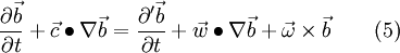
<math> \frac{\partial\vec{b}}{\partial t} + \vec{c} \bullet \nabla \vec{b} = \frac{\partial^\prime\vec{b}}{\partial t} + \vec{w} \bullet \nabla \vec{b} + \vec{\omega} \times \vec{b} \qquad (5)</math> | <math> \frac{\partial\vec{b}}{\partial t} + \vec{c} \bullet \nabla \vec{b} = \frac{\partial^\prime\vec{b}}{\partial t} + \vec{w} \bullet \nabla \vec{b} + \vec{\omega} \times \vec{b} \qquad (5)</math> | ||
| + | |||
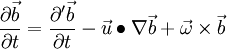
| + | With the relationship of eq. 14 this yields to | ||
| + | |||
| + | <math> \frac{\partial\vec{b}}{\partial t} = \frac{\partial^\prime\vec{b}}{\partial t} - \vec{u} \bullet \nabla \vec{b} + \vec{\omega} \times \vec{b}</math> | ||
Additional, the following identities are valid with any vector <math> \vec{a} </math> and a scalar <math> \alpha </math> [http://en.wikipedia.org/wiki/Dyadic_product#Identities] | Additional, the following identities are valid with any vector <math> \vec{a} </math> and a scalar <math> \alpha </math> [http://en.wikipedia.org/wiki/Dyadic_product#Identities] | ||
| Line 121: | Line 125: | ||
<math> \vec{c} \otimes \vec{w} \boldsymbol{\neq} \vec{w} \otimes \vec{c}</math> | <math> \vec{c} \otimes \vec{w} \boldsymbol{\neq} \vec{w} \otimes \vec{c}</math> | ||
| + | |||
| + | == Shear Stress Tensor == | ||
| + | |||
| + | |||
== References == | == References == | ||
* FLUENT 6.3 User's Guide; [http://my.fit.edu/itresources/manuals/fluent6.3/help/html/ug/node416.htm "Equations for a Rotating Reference Frame"]; Chap. 10.2.2 | * FLUENT 6.3 User's Guide; [http://my.fit.edu/itresources/manuals/fluent6.3/help/html/ug/node416.htm "Equations for a Rotating Reference Frame"]; Chap. 10.2.2 | ||
Revision as of 15:50, 7 March 2010
Contents
1 Momentum Equation
1.1 Some mathematical useful identities
The first time derivation of any vector  formulated in the absolute and relative frame of reference, according to [1], where
  is the angular frequency between these two coordinate systems. Any quantity with an ' is related to the relative frame of reference.

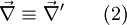
If  is a vector operator, then it is valid
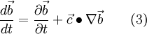
Therefor the total time derivation of any vector can be split off into a local term and a convective term. In the absolute frame of reference it gives with the absolute velocity 
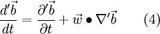
And in the relative frame of reference it gives with the relative velocity 
If we insert eq. 2-4 into the 1, one can write
With the relationship of eq. 14 this yields to
Additional, the following identities are valid with any vector  and a scalar
  [2]
[2]

and [3]

and [4]

1.2 Derivation
We are now deriving the momentum equation in the relative coordinate system but formulated with the absolute velocity.
If we use eq. 6, then it can be easily shown, that the following statement is valid

If we use the solution from eq. 9, and apply them to eq. 7, the following can be shown
![\begin{array}{rcl}
\nabla \bullet \left[ \left( \varrho \vec{c} \right) \otimes \vec{c} \right] & = &
\left[\nabla \bullet \left( \varrho \vec{c} \right)\right] \vec{c} + \left( \varrho \vec{c} \right) \bullet \nabla \vec{c} \qquad (10)\\
= \nabla \bullet \left[ \vec{c} \otimes \left( \varrho \vec{c} \right) \right] & = &
\left[\nabla \bullet \vec{c} \right] \left( \varrho \vec{c} \right) + \vec{c} \bullet \nabla \left( \varrho \vec{c} \right) \qquad (11)
\end{array}](/images/math/6/d/5/6d558ffa15615010ec9ca0f028765c46.png)
Furthermore, if we apply  in eq. 5, this gives us

Now we add the first term on the right hand side of eq. 11 ![\left[\nabla \bullet \vec{c} \right] \left( \varrho \vec{c} \right)](/images/math/6/4/5/645bc88e0975d376a8c024ab224aa1f2.png) to eq. 12 and apply furthermore eq. 11. Then it follows
to eq. 12 and apply furthermore eq. 11. Then it follows
![\begin{array}{rcl}
\dfrac{\partial \left( \varrho \vec{c} \right)}{\partial t} + \left[\nabla \bullet \vec{c} \right] \left( \varrho \vec{c} \right) + \vec{c} \bullet \nabla \left( \varrho \vec{c} \right)
& = & \dfrac{\partial^\prime\left( \varrho \vec{c} \right)}{\partial t} + \vec{w} \bullet \nabla \left( \varrho \vec{c} \right) + \vec{\omega} \times \left( \varrho \vec{c} \right) + \left[\nabla \bullet \vec{c} \right] \left( \varrho \vec{c} \right) \\
= \dfrac{\partial \left( \varrho \vec{c} \right)}{\partial t} + \nabla \bullet \left[ \left( \varrho \vec{c} \right) \otimes \vec{c} \right] & = & \dfrac{\partial^\prime\left( \varrho \vec{c} \right)}{\partial t} + \vec{\omega} \times \left( \varrho \vec{c} \right) + \underbrace{\vec{w} \bullet \nabla \left( \varrho \vec{c} \right) + \left[\nabla \bullet \vec{c} \right] \left( \varrho \vec{c} \right)}_{A1} \\
\end{array} \qquad (13)](/images/math/7/b/f/7bfaad0cd0468b155ba4ab7f526c2ca4.png)
Consider, that the origin of the absolute and relative frame of reference or coincident. Then it is valid to say, that the position vector is equal in both systems  . But, be aware, the components of these vectors are not equal, because they are defined in different base systems. If we now use
  in eq. 1, it gives usthe well known relation between the absolute and relative velocity.

If we now use the solution from eq. 14 and apply this to the first term on the right hand side of eq. 11, the following is valid
![\begin{array}{rcl}
\left[\nabla \bullet \vec{c} \right] \left( \varrho \vec{c} \right)
& = & \left[\nabla \bullet \left( \vec{w}+\vec{u} \right) \right] \left( \varrho \vec{c} \right) \\
& = & \left[\nabla \bullet \vec{w} \right] \left( \varrho \vec{c} \right) + \underbrace{\left[\nabla \bullet \left( \vec{\omega} \times \vec{r}^\prime \right)\right]}_{A2} \left( \varrho \vec{c} \right)
\end{array}\qquad (15)](/images/math/6/8/9/68901056a6d9cef87974929eaf07ccd5.png)
If we now apply eq. 8 to the term A2 of eq. 15, we get
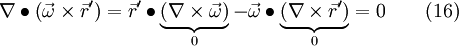
If you consider for example 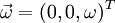 and
and 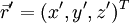 in cartesian coordinates and apply the cross product component-by-component, then the result from eq. 16 maybe become a little bit more clearer. With eq. 16, eq. 15 becomes
![\left[\nabla \bullet \vec{c} \right] \left( \varrho \vec{c} \right) = \left[\nabla \bullet \vec{w} \right] \left( \varrho \vec{c} \right) \qquad (17)](/images/math/1/9/5/195ae799f50945f325219041d7048d28.png)
Now with eq. 17 and eq. 7 term A1 from eq. 13 writes to
![\begin{array}{rcl}
\left[\nabla \bullet \vec{c} \right] \left( \varrho \vec{c} \right) + \vec{w} \bullet \nabla \left( \varrho \vec{c} \right) & = & \left[\nabla \bullet \vec{w} \right] \left( \varrho \vec{c} \right) + \vec{w} \bullet \nabla \left( \varrho \vec{c} \right) \\
& = & \nabla \bullet \left[ \vec{w} \otimes \left( \varrho \vec{c} \right) \right]
\end{array}\qquad (18)](/images/math/1/7/0/1708cac6f37df04c88ff377b56a5ba65.png)
If we now insert eq. 18 into eq. 13, we get
![\dfrac{\partial \left( \varrho \vec{c} \right)}{\partial t} + \nabla \bullet \left[ \left( \varrho \vec{c} \right) \otimes \vec{c} \right] = \dfrac{\partial^\prime\left( \varrho \vec{c} \right)}{\partial t} + \nabla \bullet \left[ \vec{w} \otimes \left( \varrho \vec{c} \right) \right] +
\vec{\omega} \times \left( \varrho \vec{c} \right)\qquad (19)](/images/math/6/e/4/6e495172aca9530cb76c8faed6548615.png)
The momentum equation of an inertial coordinate system is equal to
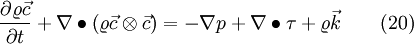
If we now apply eq. 19 to eq. 20 we get the momentum equation in a relative coordinate system, see also but not limited to ref. 1, 2, 3

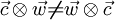
Furthermore it can be shown that the tensor 2. rank from the dyadic product of  is not symmetric, if you write it down component-by-component in cartesian coordinates. So that it must be valid to write
2 Shear Stress Tensor
3 References
- FLUENT 6.3 User's Guide; "Equations for a Rotating Reference Frame"; Chap. 10.2.2