SimpleFoam

SimpleFoam

SimpleFoam is a steady-state solver for incompressible, turbulent flow, using the SIMPLE (Semi-Implicit Method for Pressure Linked Equations) algorithm. In the newer releases it also includes an option to use the SIMPLEC (Semi-Implicit Method for Pressure Linked Equations Consistent) algorithm.

1 Solution Strategy

The solver follows a segregated solution strategy. This means that the equations for each variable characterizing the system (the velocity $\bold u$, the pressure $p$ and the variables characterizing turbulence) is solved sequentially and the solution of the preceding equations is inserted in the subsequent equation. The non-linearity appearing in the momentum equation (the face flux $\phi_f$ which is a function of the velocity) is resolved by computing it from the velocity and pressure values of the preceding iteration. The dependence from the pressure is introduced to avoid a decoupling between the momentum and pressure equations and hence the appearance of high frequency oscillation in the solution (check board effect). The first equation to be solve is the momentum equation. It delivers a velocity field $\bold u^*$ which is in general not divergence free, i.e. it does not satisfy the continuity equation. After that the momentum and the continuity equations are used to construct an equation for the pressure. The aim is to obtain a pressure field $p^{n}$, which, if inserted in the momentum equation, delivers a divergence free velocity field $\bold u$. After correcting the velocity field, the equations for turbulence are solved. The above iterative solution procedure is repeated until convergence.

The source code can be found in simpleFoam.C

 
 
/*---------------------------------------------------------------------------*\
  =========                 |
  \\      /  F ield         | OpenFOAM: The Open Source CFD Toolbox
   \\    /   O peration     | Website:  https://openfoam.org
    \\  /    A nd           | Copyright (C) 2011-2018 OpenFOAM Foundation
     \\/     M anipulation  |
-------------------------------------------------------------------------------
License
    This file is part of OpenFOAM.
 
    OpenFOAM is free software: you can redistribute it and/or modify it
    under the terms of the GNU General Public License as published by
    the Free Software Foundation, either version 3 of the License, or
    (at your option) any later version.
 
    OpenFOAM is distributed in the hope that it will be useful, but WITHOUT
    ANY WARRANTY; without even the implied warranty of MERCHANTABILITY or
    FITNESS FOR A PARTICULAR PURPOSE.  See the GNU General Public License
    for more details.
 
    You should have received a copy of the GNU General Public License
    along with OpenFOAM.  If not, see <http://www.gnu.org/licenses/>.
 
Application
    simpleFoam
 
Description
    Steady-state solver for incompressible, turbulent flow, using the SIMPLE
    algorithm.
 
\*---------------------------------------------------------------------------*/
 
#include "fvCFD.H"
#include "singlePhaseTransportModel.H"
#include "turbulentTransportModel.H"
#include "simpleControl.H"
#include "fvOptions.H"
 
// * * * * * * * * * * * * * * * * * * * * * * * * * * * * * * * * * * * * * //
 
int main(int argc, char *argv[])
{
    #include "postProcess.H"
 
    #include "setRootCaseLists.H"
    #include "createTime.H"
    #include "createMesh.H"
    #include "createControl.H"
    #include "createFields.H"
    #include "initContinuityErrs.H"
 
    turbulence->validate();
 
    // * * * * * * * * * * * * * * * * * * * * * * * * * * * * * * * * * * * //
 
    Info<< "\nStarting time loop\n" << endl;
 
    while (simple.loop(runTime))
    {
        Info<< "Time = " << runTime.timeName() << nl << endl;
 
        // --- Pressure-velocity SIMPLE corrector
        {
            #include "UEqn.H"
            #include "pEqn.H"
        }
 
        laminarTransport.correct();
        turbulence->correct();
 
        runTime.write();
 
        Info<< "ExecutionTime = " << runTime.elapsedCpuTime() << " s"
            << "  ClockTime = " << runTime.elapsedClockTime() << " s"
            << nl << endl;
    }
 
    Info<< "End\n" << endl;
 
    return 0;
}
 
 
// ************************************************************************* //
 
 

2 Equations

2.1 Momentum Equation

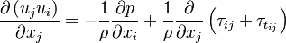$\frac{\partial \left( {u}_j u_i \right) }{\partial x_j}= - \frac{1}{\rho}\frac{\partial p} {\partial{x_i}} + \frac{1}{\rho}\frac{\partial}{\partial x_j} \left( \tau_{ij} + \tau_{t_{ij}} \right)$

(1)

$u$ represent the velocity and $\tau_{ij}$ and $\tau_{t_{ij}}$ are the viscose and turbulent stresses. Not that in simpleFoam the momentum equation solve, is divided by the constant density $\rho$.

The source code can be found in UEqn.H:

 
 
        // Momentum predictor
 
    MRF.correctBoundaryVelocity(U);
 
    tmp<fvVectorMatrix> tUEqn
    (
        fvm::div(phi, U)
      + MRF.DDt(U)
      + turbulence->divDevReff(U)
     ==
        fvOptions(U)
    );
    fvVectorMatrix& UEqn = tUEqn.ref();
 
    UEqn.relax();
 
    fvOptions.constrain(UEqn);
 
    if (simple.momentumPredictor())
    {
        solve(UEqn == -fvc::grad(p));
 
        fvOptions.correct(U);
    }
 

In the following the numeric used to solve the momentum equation are briefly explained. The first step performed is to assemble the matrix which is later solved to obtain the estimate of the velocity $\bold u^*$:

 
    tmp<fvVectorMatrix> tUEqn
    (
        fvm::div(phi, U)
      + MRF.DDt(U)
      + turbulence->divDevReff(U)
     ==
        fvOptions(U)
    );
 

In the usual semi discrete form it can be written as (see also . ):

$\bold{a_P u_P} + \sum_{N} \bold{a_N u_N} = \bold b_P$

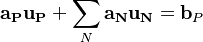(1)

$\bold a_P$ are the matrix coefficient associated with the centre point P, $\bold a_N$ the matrix coefficients associated with all neighbours influencing the computational stencil around point P and $\bold b_P$ is the source therm. The sum $\sum_N$ is taken over all neighbours influencing the computational stencil around point P.

The next step performed is the under relax the equation:

 
    UEqn.relax();

 The under relaxation is required in order to prevent the solution to diverge. Even though the discrete equation of the momentum

equation is linear, the non linearity is resolve by using the solution of the previous iteration. This causes a large change of the new velocity leading often to divergence . Using Patankar's implicit under relaxation the new semi discrete momentum equation can be written as:

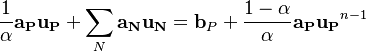$\frac{1}{\alpha}\bold{a_P u_P} + \sum_{N} \bold{a_N u_N} = \bold b_P + \frac{1 - \alpha}{\alpha}\bold{a_P u_P}^{n-1}$

(1)

Here $\alpha$ denotes the under relaxation factor and $\bold{u_P}^{n-1}$ denotes the solution at the previous iteration step. The source code for the under relaxation can be found in fvMatrix.C (see also https://www.openfoam.com/documentation/cpp-guide/html/fvMatrix_8C_source.html):

 
 
   template<class Type>
 void Foam::fvMatrix<Type>::relax(const scalar alpha)
 {
     if (alpha <= 0)
     {
         return;
     }
 
     if (debug)
     {
         InfoInFunction
             << "Relaxing " << psi_.name() << " by " << alpha << endl;
     }
 
     Field<Type>& S = source();
     scalarField& D = diag();
 
     // Store the current unrelaxed diagonal for use in updating the source
     scalarField D0(D);
 
     // Calculate the sum-mag off-diagonal from the interior faces
     scalarField sumOff(D.size(), 0.0);
     sumMagOffDiag(sumOff);
 
     // Handle the boundary contributions to the diagonal
     forAll(psi_.boundaryField(), patchi)
     {
         const fvPatchField<Type>& ptf = psi_.boundaryField()[patchi];
 
         if (ptf.size())
         {
             const labelUList& pa = lduAddr().patchAddr(patchi);
             Field<Type>& iCoeffs = internalCoeffs_[patchi];
 
             if (ptf.coupled())
             {
                 const Field<Type>& pCoeffs = boundaryCoeffs_[patchi];
 
                 // For coupled boundaries add the diagonal and
                 // off-diagonal contributions
                 forAll(pa, face)
                 {
                     D[pa[face]] += component(iCoeffs[face], 0);
                     sumOff[pa[face]] += mag(component(pCoeffs[face], 0));
                 }
             }
             else
             {
                 // For non-coupled boundaries add the maximum magnitude diagonal
                 // contribution to ensure stability
                 forAll(pa, face)
                 {
                     D[pa[face]] += cmptMax(cmptMag(iCoeffs[face]));
                 }
             }
         }
     }
 
 
     if (debug)
     {
         // Calculate amount of non-dominance.
         label nNon = 0;
         scalar maxNon = 0.0;
         scalar sumNon = 0.0;
         forAll(D, celli)
         {
             scalar d = (sumOff[celli] - D[celli])/mag(D[celli]);
 
             if (d > 0)
             {
                 nNon++;
                 maxNon = max(maxNon, d);
                 sumNon += d;
             }
         }
 
         reduce(nNon, sumOp<label>(), UPstream::msgType(), psi_.mesh().comm());
         reduce
         (
             maxNon,
             maxOp<scalar>(),
             UPstream::msgType(),
             psi_.mesh().comm()
         );
         reduce
         (
             sumNon,
             sumOp<scalar>(),
             UPstream::msgType(),
             psi_.mesh().comm()
         );
         sumNon /= returnReduce
         (
             D.size(),
             sumOp<label>(),
             UPstream::msgType(),
             psi_.mesh().comm()
         );
 
         InfoInFunction
             << "Matrix dominance test for " << psi_.name() << nl
             << "    number of non-dominant cells   : " << nNon << nl
             << "    maximum relative non-dominance : " << maxNon << nl
             << "    average relative non-dominance : " << sumNon << nl
             << endl;
     }
 
 
     // Ensure the matrix is diagonally dominant...
     // Assumes that the central coefficient is positive and ensures it is
     forAll(D, celli)
     {
         D[celli] = max(mag(D[celli]), sumOff[celli]);
     }
 
     // ... then relax
     D /= alpha;
 
     // Now remove the diagonal contribution from coupled boundaries
     forAll(psi_.boundaryField(), patchi)
     {
         const fvPatchField<Type>& ptf = psi_.boundaryField()[patchi];
 
         if (ptf.size())
         {
             const labelUList& pa = lduAddr().patchAddr(patchi);
             Field<Type>& iCoeffs = internalCoeffs_[patchi];
 
             if (ptf.coupled())
             {
                 forAll(pa, face)
                 {
                     D[pa[face]] -= component(iCoeffs[face], 0);
                 }
             }
             else
             {
                 forAll(pa, face)
                 {
                     D[pa[face]] -= cmptMin(iCoeffs[face]);
                 }
             }
         }
     }
 
     // Finally add the relaxation contribution to the source.
     S += (D - D0)*psi_.primitiveField();
 }

After the under relaxation the contribution of the pressure gradient is added to the right hand side of the matrix and the system is solve:

 
        solve(UEqn == -fvc::grad(p));

The equation in semi discrete form looks as follows:

$\frac{1}{\alpha}\bold{a_P u_P} + \sum_{N} \bold{a_N u_N} = \bold b_P + \frac{1 - \alpha}{\alpha}\bold{a_P u_P}^{n-1} - \nabla p_P$

(1)

$\nabla p_p$ denotes the contribution of the pressure gradient to the equation of the cell centre p. It depends on the scheme chosen to discretize the gradient operator.

Important for the understanding of the later described pressure equation is that the contribution of the pressure equation is not added to the source therm of the matrix object UEqn. Rather a new fvMatrix object is returned by the call of the overloaded operator == to the function solve:

 
        UEqn == -fvc::grad(p)

The function solve is then executed, which solves the new fvMatrix object in order to obtain the estimate $\bold u^*$ by also considering the contribution of the pressure equation. Note that the the volVectorField U is modified by solving the matrix since the solution vector $\psi$ of the matrix is a reference to U. An explanation of the the implementation can be found also in https://www.cfd-online.com/Forums/openfoam/213566-why-solve-ueqn-fvc-grad-p-ueqn-source-not-modified-ueqn-h-chang.html.

2.2 Pressure Equation

In this section the pressure equation solved in simpleFoam in order to ensure the mass conservation is derived. A good explanation of the derivation of the SIMPLE and also SIMPLEC method in simpleFoam can be found also in http://hobbyfoam.blogspot.com/2016/01/simplec-algorithm-of-openfoam.html.

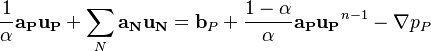
Starting point for the derivation of the pressure equation is the momentum equation in semi discrete form after the solution of the momentum equation:

$\bold{a_P^* u_P^*} = - \sum_{N} \bold{a_N u_N^*} + \bold b_P + \frac{1 - \alpha}{\alpha}\bold{a_P u_P}^{n-1} - \nabla p_P^{n-1} = \bold {H[u^*] } - \nabla p_P^{n-1}$

(1)

After dividing the above equation by $a_P^*$ we obtain:

$\bold{u_P^*} = \frac{\bold {H[u^*] }}{a_P^* } - \frac{\nabla p_P^{n-1}}{a_P^* }$

(1)

$a_P^* = \frac{1}{\alpha}a_P$ are the modified diagonal coefficients of the matrix after the under relaxation.

The scope of the next step is to find a correction for the velocity $\bold u_p'$ and for the pressure $p'$ in order to find a velocity $\bold u_p = \bold u_p^* + \bold u_p'$ which satisfies the continuum equation:

$\bold{u_P} = \frac{\bold {H[u^*] }}{a_P^* } + \frac{\bold {H[u'] }}{a_P^* } + \frac{\nabla p_P^{n-1}}{a_P^* } + \frac{\nabla p_P'}{a_P^* }$

(1)

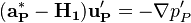
The equation for the velocity correction can be written as:

$\bold{u_P'} = - \frac{\sum_{N} \bold{a_N u_N'}}{a_P^* } - \frac{\nabla p_P'}{a_P^* } = \frac{\bold {H[u'] }}{a_P^* } - \frac{\nabla p_P'}{a_P^* }$

(1)

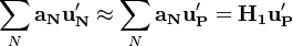
Note that here it is assumed that the diagonal coefficients of the corrector equation are the same as in the momentum equation previously solved. Taking the divergence of the above equation and setting it to zero (we want to obtain a velocity field $\bold{u_P}$ which satisfies the continuity equation) we get an equation for the pressure $p_p = p_p^{n-1} + p_p'$:

$\sum_f \frac{\bold {H[u^*] }}{a_P^* }|_f \cdot S_f + \sum_f \frac{\bold {H[u'] }}{a_P^* }|_f \cdot S_f + \sum_f \frac{\nabla p_P}{a_P^* }|_f \cdot S_f = 0$

(1)

$|_f$ denotes the values evaluated at the face.

2.2.1 Simple

If we neglect the contribution of the neighbours of the velocity correction (i.e. we set $\bold {H[u'] } = 0$) we get the pressure equation solved in the simplec algorithm:

$\sum_f \frac{\bold {H[u^*] }}{a_P^* }|_f \cdot S_f + \sum_f \frac{\nabla p_P}{a_P^* }|_f \cdot S_f = 0$

(1)

2.2.2 Simplec

The starting point for the simplec algorithm is the equation for the velocity correction. The goal is the obtain a simplification to get an explicit relation for the velocity correction and hence avoiding to solve a matrix equation:

$\sum_{N} \bold{a_N u_N'} \approx \sum_{N} \bold{a_N u_P'} = \bold{H_1 u_P'}$

(1)

Inserting the above approximation into the equation for the velocity correction we get:

$\bold{(a_P^* - H_1) u_P'} = - \nabla p_P'$

(1)

Solving for the velocity correction:

$\bold{ u_P'} = - \frac{1}{a_P^* - H_1 }\nabla p_P'$

(1)

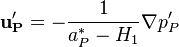
The above equation formulates an explicit relation between velocity and pressure equation. In the next step we write down:

$\bold {u_P^*} + \bold{ u_P'} = \frac{\bold {H[u^*] }}{a_P^* } - \frac{\nabla p_P^{n-1}}{a_P^* } - \frac{1}{a_P^* - H_1 }\nabla p_P' = \frac{\bold {H[u^*] }}{a_P^* } - \left ( \frac{1}{a_P^*} - \frac{1}{a_P^* - H_1 } \right )\nabla p_P^{n-1} - \frac{1}{a_P^* }\nabla p_P$

(1)

By taking the divergence of the above equation and setting it to zero we obtain the pressure equation for the simplec algorithm:

$\sum_f \frac{\bold {H[u^*] }}{a_P^* }|_f \cdot S_f - \sum_f \left ( \frac{1}{a_P^*} |_f - \frac{1}{a_P^* |_f - H_1 |_f } \right )\nabla p_P^{n-1} |_f \cdot S_f - \sum_f \frac{1}{a_P^* }\nabla p_P |_f \cdot S_f = 0$

(1)

The difference between the pressure equation in the SIMPLE and SIMPLEC consists only in one term.

The source code for the pressure equation can be seen here:

 
 
    volScalarField rAU(1.0/UEqn.A());
    volVectorField HbyA(constrainHbyA(rAU*UEqn.H(), U, p));
    surfaceScalarField phiHbyA("phiHbyA", fvc::flux(HbyA));
    MRF.makeRelative(phiHbyA);
    adjustPhi(phiHbyA, U, p);
 
    tmp<volScalarField> rAtU(rAU);
 
    if (simple.consistent())
    {
        rAtU = 1.0/(1.0/rAU - UEqn.H1());
        phiHbyA +=
            fvc::interpolate(rAtU() - rAU)*fvc::snGrad(p)*mesh.magSf();
        HbyA -= (rAU - rAtU())*fvc::grad(p);
    }
 
    tUEqn.clear();
 
    // Update the pressure BCs to ensure flux consistency
    constrainPressure(p, U, phiHbyA, rAtU(), MRF);
 
    // Non-orthogonal pressure corrector loop
    while (simple.correctNonOrthogonal())
    {
        fvScalarMatrix pEqn
        (
            fvm::laplacian(rAtU(), p) == fvc::div(phiHbyA)
        );
 
        pEqn.setReference(pRefCell, pRefValue);
 
        pEqn.solve();
 
        if (simple.finalNonOrthogonalIter())
        {
            phi = phiHbyA - pEqn.flux();
        }
    }
 
    #include "continuityErrs.H"
 
    // Explicitly relax pressure for momentum corrector
    p.relax();
 
    // Momentum corrector
    U = HbyA - rAtU()*fvc::grad(p);
    U.correctBoundaryConditions();
    fvOptions.correct(U);
}
 
 

2.3 Avoiding checker boarder effects

The usual way to avoid the so called "checker board" effect is to interpolate the velocities at the faces by means of the Rhie and Chow interpolation (see e.g. or . ) . The checker board effect has its origin in the absence of neighbouring pressure terms in the momentum equation due to the discretization of the pressure gradient term in the frame of the finite volume method. The same absence of neighbouring pressure terms is obtained when the Laplacian term is discretized by linear interpolation of the pressure gradient on the face centres. In the implementation of the simpleFoam solver, the Rhie and Chow interpolation is not done in an explicit way. The introduction of neighbour pressure terms in the momentum and pressure equation is done in the spirit of Rhie and Chow . It is achieved by two contribution: The first one is the way the Laplacian term is disretized (see also http://www.tfd.chalmers.se/~hani/kurser/OS_CFD_2007/rhiechow.pdf). The second contribution is achieved by the flux() operator after the solution of the pressure equation:

 
        if (simple.finalNonOrthogonalIter())
        {
            phi = phiHbyA - pEqn.flux();
        }

The principle of how the pressure oscillations are avoided in simpleFoam are explained by means of a simple 1D convection equation:

$\frac{\partial \left( \rho {u} u \right) }{\partial x}= -\frac{\partial p} {\partial{x}}$

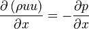(x)

The above equation is to be discretized on a equidistant grid:

 
 
----------------------------------------------------------------------------------------------------------------------------- 
|                        |                         |                        |                        |                        |
|                        |                         |                        |                        |                        |      
|         WW             |ww       W               |w        P             e|          E          ee |               EE       |
|                        |                         |                        |                        |                        |
|                        |                         |                        |                        |                        |
-----------------------------------------------------------------------------------------------------------------------------
 

The usual geographic notation is adoped to describe the discretization stencil around the point P for which the solution has to be obtained.

The discretization with a finite volume method leads to the following equation:

$\sum_f \phi_f u_f = -\sum_f p_f S_f$

(x)

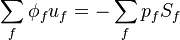
$\phi_f$ is the phase flux and is computed from the previous iteration in order to resolve the non-linearity in the momentum equation. Evaluating the above sum for the central point P we get:

$\phi_e u_e - \phi_w u_w = - (p_e - p_w) \Delta y$

(x)

With a central discretization of the velocity and pressure at the faces we obtain:

$\phi_e \frac{1}{2} (u_P + u_E) - \phi_w \frac{1}{2} ( u_P + u_W) = - \left(\frac{1}{2}(p_P + p_E) - \frac{1}{2} (p_P + p_W) \right) \Delta y$

(x)

And finally:

$u_P \underbrace{ (\phi_e - \phi_w )}_{a_P} + \underbrace{u_E \phi_e - u_W \phi_w}_{\bold H[u]} = - \left ( p_E - p_W \right) \Delta y$

(x)

It is evident that if no spatial care is taken and the face flux $\phi_f$ is obtained by linear interpolation of the velocities the velocity at the cell center P is not coupled with the pressure at P but only at the neighboring points E and W. The diagonal coefficient $\bold a_P$ are in this case 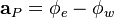$\bold a_P = \phi_e - \phi_w$ and the contributions of the neighbor cells $\bold H[u]$ are $\bold H[u] = u_E \phi_e - u_W \phi_w$ .

In order to understand how the pressure at the cell centre P is cast into the momentum equation it is important to understand how the flux() operator is defined in the fvMatrix class. Note that a very good description can be found in https://www.cfd-online.com/Forums/openfoam/114933-description-flux-method.html. Using the implementation of the flux operator we get the new fluxes at the faces for this example:

$\phi_e = \bold{ \frac{H[u^{-}]}{a_p^-}}|_e - \frac{p_P - p_E}{\Delta x \bold a_P^-|e}$

(x)

$\phi_w = \bold{ \frac{H[u^-]}{a_p^-}}|_w - \frac{p_W - p_P}{\Delta x \bold a_P^-|w}$

(x)

Note that the quantities denoted with ${^-}$ denote the quantities at the previous iteration and $\Delta x = 1$ in this illustriously example. Note also that the pressure used to correct the face fluxes come from the solution of the pressure equation. After inserting the two above relations for the phase fluxes on the east and west side of the cell centre in the momentum equation we get:

$u_P \left ( \bold{ \frac{H[u^{-}]}{a_p^-}}|_e - \bold{ \frac{H[u^-]}{a_p^-}}|_w - \frac{p_P - p_E}{\Delta x \bold a_P^-|e} + \frac{p_W - p_P}{\Delta x \bold a_P^-|w} \right ) + u_E\left( \bold{ \frac{H[u^{-}]}{a_p^-}}|_e - \frac{p_P - p_E}{\Delta x \bold a_P^-|e} \right ) - u_W \left ( \bold{ \frac{H[u^-]}{a_p^-}}|_w - \frac{p_W - p_P}{\Delta x \bold a_P^-|w} \right ) = - \left ( p_E - p_W \right) \Delta y$

(x)

It evident that by correcting the face fluxes with the flux() operator of the fvMatrix class we obtain a dependency of the velocity at the centre point P from the pressure at the centre point P.