Difference between revisions of "BubbleFoam"
(→Solution procedure) |
m (→Solution procedure) |
||
| Line 161: | Line 161: | ||
#Predict the phase velocity fields, without considering the pressure gradient at this stage | #Predict the phase velocity fields, without considering the pressure gradient at this stage | ||
#Solve the pressure equation | #Solve the pressure equation | ||
| − | #Correct the velocities with the new pressure field, and update | + | #Correct the velocities with the new pressure field, and update the phase fractions |
| − | the phase fractions | + | |
#Solve the transport equations for the turbulence quantities | #Solve the transport equations for the turbulence quantities | ||
Revision as of 04:28, 12 February 2010
Valid versions: ![]()
Contents
- 1 Introduction and applications
- 2 bubbleFoam capabilities and limitations
- 3 bubbleFoam theory
- 4 bubbleFoam implementation
- 5 bubbleFoam setup and solution strategy
- 6 References
1 Introduction and applications
The bubbleFoam solver is a two-phase solver based on the Euler-Euler two-fluid methodology [1, 2, 3, 4, 10], suitable to compute dispersed gas-liquid and liquid-liquid flows. In the Euler-Euler two-fluid approach, the phases are treated as interpenetrating continua, which are capable of exchanging properties, like momentum, energy and mass one with the other. Typical applications of the two-fluid approach, as implemented in bubbleFoam, are:
- bubble columns
- stirred tank reactors
- static mixers
2 bubbleFoam capabilities and limitations
2.1 bubbleFoam capabilities
The bubbleFoam solver implements the two-fluid equations derived in [10, 8] for the simulation of gas-liquid flows. The model undergoes the following assumptions:
- Phases are incompressible
- The dispersed phase particle diameter is constant
- The flow is isothermal
- Only momentum exchange is accounted for in the momentum transport equations
The main features of the solver are the following:
- Capability to solve for dispersed two-phase flows with strong density ratio
- Robust solution algorithm, able to deal with complete flow separation
- Turbulence modelling through κ − ε model and standard wall functions.
2.2 bubbleFoam limitations
The bubbleFoam solver currently has the following limitations:
- Only one dispersed phase and a continuous phase can be described. It is not possible to account for multiple dispersed phases (i.e. represent a dispersed phase diameter distribution)
- The diameter of the particles1 constituting the dispersed phase is assumed to be constant. Aggragation, breakage and coalescence phenomena are not accounted for
- The drag coefficient is computed as a blend of the drag coefficients evaluated for each phase on the basis of the phase fractions, and no alternative drag models are available
- The interaction between the phases happens only through the momentum exchange term in the corresponding momentum equations:
- It is not possible to model the heat transfer between the phases
- It is not possible to model the mass transfer between the phases
- No chemical reaction model is available.
3 bubbleFoam theory
3.1 Overview
The two-fluid equations solved by the bubbleFoam solver are described in this chapter. The general two-fluid continuity and momentum equations are introduced, the closure expressions for the phase stress tensor and the momentum transfer term are presented, and the transport equations of the turbulence model are summarized.
3.2 Governing equations
In the two-fluid approach, a continuity and a momentum equation are solved for each
phase present in the system. These equations can be derived by conditionally averaging
the single phase flow equations. The reader interested in the theoretical background is
invited to refer to, for example, [1, 2, 3, 10].
The continuity equations for each phase  has the form
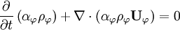
where  represents the phase fraction of phase ,
  is the density of the material
constituting the same phase, and
is the density of the material
constituting the same phase, and  is the phase velocity.
The phase momentum equation is
is the phase velocity.
The phase momentum equation is

in which  is the phase laminar stress tensor, assumed to be Newtonian,
  is the phase
Reynolds stress tensor,
is the phase
Reynolds stress tensor,  is the pressure,
  is the gravitational acceleration vector, and
  is the momentum exchange term.
The laminar stress tensor is defined, for each phase, as
is the momentum exchange term.
The laminar stress tensor is defined, for each phase, as
![\boldsymbol{\tau}_{\varphi} = - \rho_{\varphi} \nu_{\varphi} \left[\nabla \mathbf{U}_{\varphi} + \nabla^{\textrm{T}} \mathbf{U}_{\varphi} \right] + \frac{2}{3}\rho_{\varphi}\nu_{\varphi} \left( \nabla \cdot \mathbf{U}_{\varphi} \right) \mathbf{I}](/images/math/8/5/6/8567cc32aafb5b800824a76cf7294a1d.png)
where  is the molecular kinematic viscosity of the fluid constituting phase , and
  is
the identity matrix. The phase Reynolds stress tensor is given by
is
the identity matrix. The phase Reynolds stress tensor is given by
![\mathbf{R}_{\varphi} = - \rho_{\varphi} \nu_{\varphi,\textrm{t}} \left[ \nabla \mathbf{U}_{\varphi} +\nabla^{\textrm{T}} \mathbf{U}_{\varphi} \right] + \frac{2}{3} \rho_{\varphi} \nu_{\varphi,\textrm{t}} \left( \nabla \cdot \mathbf{U}_{\varphi} \right) \mathbf{I} + \frac{2}{3} \rho_{\varphi} \kappa_{\varphi} \mathbf{I}](/images/math/6/9/d/69db1b3ec4c80ca53d12dc833b332abe.png)
where  is the phase turbulent kinetic energy (Note that in the bubbleFoam implementation, it assumed that
  . In other words, the turbulent kinetic energy is identical for both the phases present in the system), and
  is the phase turbulent kinematic viscosity, defined as
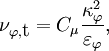
in which  is a constant, and
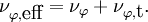
  is the phase turbulent dissipation rate. The phase effective viscosity is calculated as the sum of the phase molecular viscosity and of the phase turbulent viscosity, as
The momentum exchange term can be decomposed in a drag contribution, a lift force contribution and a virtual mass contribution

where the terms are modelled according to the mixture model [10]. In particular, indicating with a and b the two phases considered in the two-fluid model, where a represents the dispersed phase, the drag term is described by equation
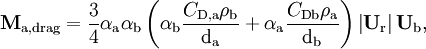
in which  and
and  are the phase particle diameters,
 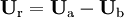 is the relative velocity vector, and
  and
and  are the drag coefficients computed with respect to each phase, according to
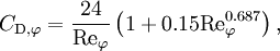
where 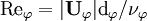 .
.
The lift for term is modelled as (Notice that  should actually be
  . We report for consistency with the code implementation.}

while the virtual mass force term is evaluated as

where
and
 .
.
3.2.1 Turbulence model
The bubbleFoam solver uses a two-equation  turbulence model for the continuous phase, and accounts for the influence of the turbulence on the dispersed phase by scaling the dispersed phase turbulent viscosity. The equation for the turbulent kinetic energy of the continuous phase (
 ) reads

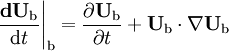
where  is the producton of the turbulent kinetic energy, given by
![G = 2 \nu_{\textrm{b},\textrm{t}} \left[ \nabla \mathbf{U}_{\textrm{b}} \cdot \operatorname{dev} \left( \nabla \mathbf{U}_{\textrm{b}} + \nabla^{\textrm{T}} \mathbf{U}_{\textrm{b}} \right) \right],](/images/math/7/6/b/76bf3e0d36fd204d7e234e6388238447.png) and
and  is the turbulent Schmidt number.
The turbulent dissipation rate is determined by solving the transport equation
is the turbulent Schmidt number.
The turbulent dissipation rate is determined by solving the transport equation

where  and
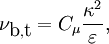
and  are constant of the turbulence model. The turbulence viscosity of the continuous phase is calculated from its definition
while the turbulent viscosity of the dispersed phase is evaluated as
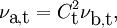
being the coefficient  and the turbulence response coefficient
  constants of the model. Standard wall functions are adopted to treat the zone next to the wall.
4 bubbleFoam implementation
The numerical solution of the two-phase equations relies on a segregated algorithm based on the PISO procedure extended to two-phase flows [5]. The momentum equations are manipulated to stabilize the system of equation at the limits of the range of volume fractions, to avoid singularities, as suggested in [5, 10]. The details of the numerical methodology are briefly summarized in this chapter.
4.1 Numerical methodology
4.1.1 Phase momentum equation
4.1.2 Phase continuity equation
4.1.3 Pressure equation
4.2 Solution procedure
The solution procedure adopted in the bubbleFoam solver is summed up as follows:
- Solve the phase continuity equations
- Update lift, drag and virtual mass coefficients
- Construct the momentum equation matrix
- Predict the phase velocity fields, without considering the pressure gradient at this stage
- Solve the pressure equation
- Correct the velocities with the new pressure field, and update the phase fractions
- Solve the transport equations for the turbulence quantities
4.3 Code representation
4.3.1 Implementation of the phase momentum equation
4.3.2 Implementation of the phase continuity equation
4.3.3 Implementation of the pressure equation
5 bubbleFoam setup and solution strategy
5.1 Case structure
5.2 Initial conditions
5.3 Solver configuration
5.3.1 The environmentalProperties dictionary
5.3.2 The RASProperties dictionary
5.3.3 The transportProperties dictionary
5.4 Solver controls
5.4.1 The controlDict dictionary
5.4.2 The fvSchemes dictionary
5.4.3 The fvSolution dictionary
6 References
- D. A. Drew. Averaged equations for two-phase flows. Studies in Applied Mathematics, L(3):205 – 231, 1971.
- D. A. Drew. Continuum modeling of two-phase flows. In R. Meyer, editor, Theory of dispersed multiphase flow, pages 173 – 190. Academic Press, 1983.
- H. Enwald, E. Peirano, and A. E. Almstedt. Eulerian two-phase flow theory applied to fluidization. International Journal of Multiphase Flow, 22:21 – 66, 1996.
- D. P. Hill. The computer simulation of dispersed two-phase flow. PhD thesis, Imperial College of Science, Technology and Medicine, London, U.K., 1998.
- J. P. Oliveira and R. I. Issa. Numerical aspects of an algorithm for Eulerian simulation of two-phase flows. International Journal for Numerical Methods in Fluids, 43:1177 – 1198, 2003.
- OpenCFD. OpenFOAM - The Open Source CFD Toolbox - Programmer’s Guide. OpenCFD Ltd., United Kingdom, 1.4 edition, 11 April 2007.
- OpenCFD. OpenFOAM - The Open Source CFD Toolbox - User’s Guide. OpenCFD Ltd., United Kingdom, 1.4 edition, 11 April 2007.
- H. Rusche. Computational fluid dynamics of dispersed two-phase flows at high phase fractions. PhD thesis, Imperial College of Science, Technology and Medicine, London, 2002.
- L. Schiller and A. Naumann. Uber die grundlegenden Berechnungen bei der Schwerkraftaufbereitung. Zeitschrift des Vereins deutscher Ingenieure, 77(12):318, 1933.
- H. G. Weller. Derivation, modelling and solution of the conditionally averaged two-phase flow equations. Technical report, OpenCFD Ltd., United Kingdom, 23 February 2005.