ChtMultiRegionFoam

ChtMultiRegionFoam

   Solver for steady or transient fluid flow and solid heat conduction, with
   conjugate heat transfer between regions, buoyancy effects, turbulence,
   reactions and radiation modelling.

1 Equations

For each region defined as fluid, the according equation for the fluid is solved and the same is done for each solid region. The regions are coupled by a thermal boundary condition. A short description of the solver can be found also in

1.1 Equations Fluid

For each fluid region the compressible Navier Stokes equation are solved. The solver used to solve the fluid equations is a pressure bases solver. That means that a pressure equation (similar to the pressure equation used in an incompressible solver) is used to establish the connection between the momentum and the continuity equation. The algorithm to advance the solution in time is the following:

1. Update the density with the help of the continuity equation

2. Solve the momentum equation

3. Solve the spices transport equation

4. Solve the energy equation

5. Solve the pressure equation to ensure mass conservation

The source code can be found in solveFluid.H

 
 
if (pimple.frozenFlow())
{
    #include "EEqn.H"
}
else
{
    if (!mesh.steady() && pimples.nCorrPimple() <= 1)
    {
        #include "rhoEqn.H"
    }
 
    #include "UEqn.H"
    #include "YEqn.H"
    #include "EEqn.H"
 
    // --- PISO loop
    while (pimple.correct())
    {
        #include "pEqn.H"
    }
 
    if (pimples.pimpleTurbCorr(i))
    {
        turbulence.correct();
    }
 
    if (!mesh.steady() && pimples.finalIter())
    {
        rho = thermo.rho();
    }
}
 

1.1.1 Mass conservation

The variable-density continuity equation is

$\frac{\partial \rho}{\partial t} + \frac{\partial {\rho u}_j}{\partial x_j} = 0$

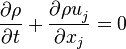(1)

The source code can be found in src/finiteVolume/cfdTools/compressible/rhoEqn.H:

 
 
{
    fvScalarMatrix rhoEqn
    (
        fvm::ddt(rho)
      + fvc::div(phi)
      ==
        fvOptions(rho)
    );
 
    fvOptions.constrain(rhoEqn);
 
    rhoEqn.solve();
 
    fvOptions.correct(rho);
}
 

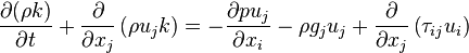
1.1.2 Momentum conservation

$\frac{ \partial (\rho {u}_i)}{\partial t} + \frac{\partial}{\partial x_j} \left( \rho {u}_j u_i \right) = - \frac{\partial p_{rgh}} {\partial{x_i}} - \frac{\partial \rho g_j x_j}{\partial x_i} + \frac{\partial}{\partial x_j} \left( \tau_{ij} + \tau_{t_{ij}} \right)$

(2)

$u$ represent the velocity, $g_i$ the gravitational acceleration, 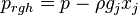$p_{rgh} = p - \rho g_j x_j$ the pressure minus the hydrostatic pressure and $\tau_{ij}$ and $\tau_{t_{ij}}$ are the viscose and turbulent stresses.

The source code can be found in Ueqn.H:

 
 
    // Solve the Momentum equation
 
    MRF.correctBoundaryVelocity(U);
 
    tmp<fvVectorMatrix> tUEqn
    (
        fvm::ddt(rho, U) + fvm::div(phi, U)
      + MRF.DDt(rho, U)
      + turbulence.divDevRhoReff(U)
     ==
        fvOptions(rho, U)
    );
    fvVectorMatrix& UEqn = tUEqn.ref();
 
    UEqn.relax();
 
    fvOptions.constrain(UEqn);
 
    if (pimple.momentumPredictor())
    {
        solve
        (
            UEqn
         ==
            fvc::reconstruct
            (
                (
                  - ghf*fvc::snGrad(rho)
                  - fvc::snGrad(p_rgh)
                )*mesh.magSf()
            )
        );
 
        fvOptions.correct(U);
        K = 0.5*magSqr(U);
    }
 
    fvOptions.correct(U);
 
 

1.1.3 Pressure equation

A good explanation of the derivation of the pressure correction equation for incompressible flows can be found in the book . In this solver however a pressure equation is solved. The purpose is to correct the velocity field and via the equation of sate also the density in order to have a velocity and density field which satisfy the continuity equation. The derivation of this pressure equation can be found in . or also following the link https://feaweb.aub.edu.lb/research/cfd/pdfs/publications/Algorithms-1.pdf.

The equation reads in semi discrete form:

$\frac{ \partial \rho}{\partial t} V_P + \sum_f \psi p v_f ^* \cdot S_f + \sum_f \rho_f^* \frac{\bold{H[v^*]}}{\bold{A_P}} \cdot S_f - \sum_f \frac{\nabla p_P}{\bold{A_P}} \cdot S_f - \sum_f \rho_f^*v_f^* \cdot S_f + \sum_f \rho_f^* \frac{\bold{H[v']}}{\bold{A_P}} \cdot S_f + \sum_f \rho_f^'v_f^' \cdot S_f = 0$

(x)

The density $\rho$ can be written as:

$\rho = \psi p$

(x)

The sum is taken over the faces of the cell with the centre point P. The last term in the above equation is very small and hence neglected. The second last term is also neglected since the velocity correction $v'$ is not know a the moment of the solution of the equation. Hence the final form of the pressure equation reads:

$\frac{ \partial \rho}{\partial t} V_P + \sum_f \psi p v_f ^* \cdot S_f + \sum_f \rho_f^* \frac{\bold{H[v^*]}}{\bold{A_P}} \cdot S_f - \sum_f \frac{\nabla p_P}{\bold{A_P}} \cdot S_f - \sum_f \rho_f^*v_f^* \cdot S_f = 0$

(x)

The pressure p can be written as

$p = p_{rgh} + \rho g_i x_i$

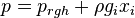(x)

The purpose is the obtain an equation for modified pressure $p_{rgh}$. Inserting the expression for the pressure in the above equation one obtains:

$\frac{ \partial \rho }{\partial t} V_P + \sum_f \psi ( p_{rgh} + \rho g_i x_i ) v_f ^* \cdot S_f + \sum_f \rho_f^* \frac{\bold{H[v^*]}}{\bold{A_P}} \cdot S_f - \sum_f \frac{\nabla p_{rghP}}{\bold{A_P}} \cdot S_f - \sum_f \frac{\nabla \rho_{P} g_i x_i}{\bold{A_P}} \cdot S_f - \sum_f \rho_f^*v_f^* \cdot S_f = 0$

(x)

.

The above equation still contains the density $\rho$ of the current time step. As approximation of the density of the current time step the density of the previous time step $\rho^*$ could be used. By doing this and with the following expression:

$\psi p_{rgh} = \psi p - \psi \rho g_i x_i = \rho - \psi \rho g_i x_i$

(x)

the above equation for the modified pressure could be simplified:

$\frac{ \partial \rho }{\partial t} V_P + \sum_f \psi p_{rgh} v_f ^* \cdot S_f - \sum_f \psi p_{rgh}^* v_f ^* \cdot S_f + \sum_f \rho_f^* \frac{\bold{H[v^*]}}{\bold{A_P}} \cdot S_f - \sum_f \frac{\nabla p_{rghP}}{\bold{A_P}} \cdot S_f - \sum_f \frac{\nabla \rho^*_{P} g_i x_i}{\bold{A_P}} \cdot S_f = 0$

(x)

.

Comparing the above equation with the source code in the bottom we can identify the corrected phase velocity without considering the pressure gradient as:

$v_f ^* = \frac{\bold{H[v^*]}}{\bold{A_P}} - \frac{\nabla \rho^*_{P} g_i x_i}{\bold{A_P}}$

(x)

.

In order to derive the expression for the time derivative in the source code of the pressure equation, the density is divided into the density of the previous time step $\rho^*$ and a density correction $\rho^'$, i.e., $\rho = \rho^* + \rho^'$ and the time derivative is taken from this expression:

$\frac{\partial \rho}{\partial t} = \frac{\partial \rho^*}{\partial t} + \frac{\partial \rho^'}{\partial t} = \frac{\partial \rho^*}{\partial t} + \psi ( \frac{\partial p_{rgh}^'}{\partial t} + \frac{\partial \rho^'}{\partial t}g_i x_i )$

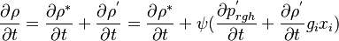(x)

.

Neglecting the last two terms in the above equation one obtains:

$\frac{\partial \rho}{\partial t} = \frac{\partial \rho^*}{\partial t} + \psi \frac{\partial p_{rgh}^'}{\partial t}$

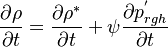(x)

.

The source code for the pressure equation can be found in pEqn.H:

 
 
if (!mesh.steady() && !pimple.simpleRho())
{
    rho = thermo.rho();
}
 
volScalarField rAU("rAU", 1.0/UEqn.A());
surfaceScalarField rhorAUf("rhorAUf", fvc::interpolate(rho*rAU));
volVectorField HbyA(constrainHbyA(rAU*UEqn.H(), U, p_rgh));
if (pimple.nCorrPISO() <= 1)
{
    tUEqn.clear();
}
 
surfaceScalarField phig(-rhorAUf*ghf*fvc::snGrad(rho)*mesh.magSf());
 
surfaceScalarField phiHbyA
(
    "phiHbyA",
    fvc::flux(rho*HbyA)
  + MRF.zeroFilter(rhorAUf*fvc::ddtCorr(rho, U, phi))
);
 
MRF.makeRelative(fvc::interpolate(rho), phiHbyA);
 
const bool closedVolume = adjustPhi(phiHbyA, U, p_rgh);
const bool adjustMass = closedVolume && !thermo.incompressible();
 
phiHbyA += phig;
 
// Update the pressure BCs to ensure flux consistency
constrainPressure(p_rgh, rho, U, phiHbyA, rhorAUf, MRF);
 
{
    fvScalarMatrix p_rghEqnComp
    (
        fvc::ddt(rho) + psi*correction(fvm::ddt(p_rgh))
    );
 
    if (pimple.transonic())
    {
        surfaceScalarField phid
        (
            "phid",
            (fvc::interpolate(psi)/fvc::interpolate(rho))*phiHbyA
        );
 
        phiHbyA -= fvc::interpolate(psi*p_rgh)*phiHbyA/fvc::interpolate(rho);
 
        p_rghEqnComp += fvm::div(phid, p_rgh);
    }
 
    // Thermodynamic density needs to be updated by psi*d(p) after the
    // pressure solution
    tmp<volScalarField> psip0(mesh.steady() ? tmp<volScalarField>() : psi*p);
 
    while (pimple.correctNonOrthogonal())
    {
        fvScalarMatrix p_rghEqnIncomp
        (
            fvc::div(phiHbyA)
          - fvm::laplacian(rhorAUf, p_rgh)
        );
 
        fvScalarMatrix p_rghEqn(p_rghEqnComp + p_rghEqnIncomp);
 
        p_rghEqn.setReference
        (
            pressureControl.refCell(),
            pressureControl.refValue()
        );
 
        p_rghEqn.solve(mesh.solver(p_rgh.select(pimple.finalInnerIter())));
 
        if (pimple.finalNonOrthogonalIter())
        {
            // Calculate the conservative fluxes
            phi = phiHbyA + p_rghEqn.flux();
 
            // Explicitly relax pressure for momentum corrector
            p_rgh.relax();
 
            // Correct the momentum source with the pressure gradient flux
            // calculated from the relaxed pressure
            U = HbyA
                + rAU*fvc::reconstruct((phig + p_rghEqnIncomp.flux())/rhorAUf);
            U.correctBoundaryConditions();
            fvOptions.correct(U);
            K = 0.5*magSqr(U);
        }
    }
 
    p = p_rgh + rho*gh;
 
    // Thermodynamic density update
    if (!mesh.steady())
    {
        thermo.correctRho(psi*p - psip0);
    }
}
 
// Update pressure time derivative if needed
if (thermo.dpdt())
{
    dpdt = fvc::ddt(p);
}
 
// Solve continuity
if (!mesh.steady())
{
    #include "rhoEqn.H"
    #include "compressibleContinuityErrs.H"
}
else
{
    #include "incompressible/continuityErrs.H"
}
 
// Pressure limiting
const bool pLimited = pressureControl.limit(p);
 
// For closed-volume compressible cases adjust the pressure level
// to obey overall mass continuity
if (adjustMass)
{
    p += (initialMass - fvc::domainIntegrate(thermo.rho()))
        /fvc::domainIntegrate(psi);
    p_rgh = p - rho*gh;
}
 
if (adjustMass || pLimited)
{
    p.correctBoundaryConditions();
}
 
// Density updates
if (adjustMass || pLimited || mesh.steady() || pimple.simpleRho())
{
    rho = thermo.rho();
}
 
if (mesh.steady() && !pimple.transonic())
{
    rho.relax();
}
 
Info<< "Min/max rho:" << min(rho).value() << ' '
    << max(rho).value() << endl;
 
 

1.1.4 Energy conservation

The energy equation can be found in: https://cfd.direct/openfoam/energy-equation/

The total energy of a fluid element can be seen as the sum of kinetic energy $k = 0.5 u_i u_i$ and internal energy $e$ . The rate of change of the kinetic energy within a fluid element is the work done on this fluid element by the viscous forces, the pressure and eternal volume forces like the gravity:

$\frac{ \partial (\rho k)}{\partial t} + \frac{\partial}{\partial x_j} \left( \rho {u}_j k \right) = - \frac{\partial p u_j} {\partial{x_i} }- \rho g_j u_j + \frac{\partial}{\partial x_j}\left( \tau_{ij} u_i \right)$

(3)

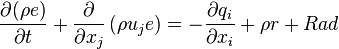
The rate of change of the internal energy $e$ of a fluid element is the heat transferred to this fluid element by diffusion and turbulence $q_i + q_{ti}$ plus the heat source term $r$ plus the heat source by radiation $Rad$  :

$\frac{ \partial (\rho e)}{\partial t} + \frac{\partial}{\partial x_j} \left( \rho {u}_j e \right) = - \frac{\partial q_i} {\partial{x_i} } + \rho r + Rad$

(4)

The change rate of the total energy is the sum of the above two equations:

$\frac{ \partial (\rho e)}{\partial t} + \frac{\partial}{\partial x_j} \left( \rho {u}_j e \right) + \frac{ \partial (\rho k)}{\partial t} + \frac{\partial}{\partial x_j} \left( \rho {u}_j k \right) = - \frac{\partial ( q_i + q_{ti}) } {\partial{x_i} } + \rho r + Rad - \frac{\partial p u_j} {\partial{x_i} }- \rho g_j u_j + \frac{\partial}{\partial x_j}\left( \tau_{ij} u_i \right)$

(5)

Instead of the internal energy $e$ there is also the option to solve the equation for the enthalpy 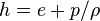$h = e + p/\rho$:

$\frac{ \partial (\rho h)}{\partial t} + \frac{\partial}{\partial x_j} \left( \rho {u}_j h \right) + \frac{ \partial (\rho k)}{\partial t} + \frac{\partial}{\partial x_j} \left( \rho {u}_j k \right) = - \frac{\partial ( q_i + q_{ti})} {\partial{x_i} } + \rho r + Rad + \frac{\partial p} {\partial{t} }- \rho g_j u_j + \frac{\partial}{\partial x_j}\left( \tau_{ij} u_i \right)$

(5)

The source code can be found in EEqn.H:

 
{
    volScalarField& he = thermo.he();
 
    fvScalarMatrix EEqn
    (
        fvm::ddt(rho, he) + fvm::div(phi, he)
      + fvc::ddt(rho, K) + fvc::div(phi, K)
      + (
            he.name() == "e"
          ? fvc::div
            (
                fvc::absolute(phi/fvc::interpolate(rho), U),
                p,
                "div(phiv,p)"
            )
          : -dpdt
        )
      - fvm::laplacian(turbulence.alphaEff(), he)
     ==
        rho*(U&g)
      + rad.Sh(thermo, he)
      + Qdot
      + fvOptions(rho, he)
    );
 
    EEqn.relax();
 
    fvOptions.constrain(EEqn);
 
    EEqn.solve();
 
    fvOptions.correct(he);
 
    thermo.correct();
    rad.correct();
 
    Info<< "Min/max T:" << min(thermo.T()).value() << ' '
        << max(thermo.T()).value() << endl;
}

1.1.5 Species conservation

In order to account for the chemical reactions occurring between different chemical species a conservation equation for each species k has to be solved:

$\frac{ \partial (\rho Y_k)}{\partial t} + \frac{\partial}{\partial x_j} \left( \rho {u}_j Y_k \right) = \frac{\partial } {\partial{x_j} }\mu_{eff}\frac{\partial Y_k}{\partial x_j} + R_k$

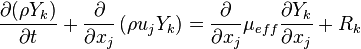(6)

$R_k$ is the reaction rate of the species k.

The source code can be found in YEqn.H:

 
tmp<fv::convectionScheme<scalar>> mvConvection(nullptr);
 
if (Y.size())
{
    mvConvection = tmp<fv::convectionScheme<scalar>>
    (
        fv::convectionScheme<scalar>::New
        (
            mesh,
            fields,
            phi,
            mesh.divScheme("div(phi,Yi_h)")
        )
    );
}
 
{
    reaction.correct();
    Qdot = reaction.Qdot();
    volScalarField Yt
    (
        IOobject("Yt", runTime.timeName(), mesh),
        mesh,
        dimensionedScalar("Yt", dimless, 0)
    );
 
    forAll(Y, i)
    {
        if (i != inertIndex && composition.active(i))
        {
            volScalarField& Yi = Y[i];
 
            fvScalarMatrix YiEqn
            (
                fvm::ddt(rho, Yi)
              + mvConvection->fvmDiv(phi, Yi)
              - fvm::laplacian(turbulence.muEff(), Yi)
             ==
                reaction.R(Yi)
              + fvOptions(rho, Yi)
            );
 
            YiEqn.relax();
 
            fvOptions.constrain(YiEqn);
 
            YiEqn.solve(mesh.solver("Yi"));
 
            fvOptions.correct(Yi);
 
            Yi.max(0.0);
            Yt += Yi;
        }
    }
 
    if (Y.size())
    {
        Y[inertIndex] = scalar(1) - Yt;
        Y[inertIndex].max(0.0);
    }
}
 

1.2 Equations Solid

For the solid regions only the energy equation has to be solved. The energy equation states that the temporal change of enthalpy of the solid is equal to the divergence of the heat conducted through the solid:

$\frac{ \partial (\rho h)}{\partial t} = \frac{\partial}{\partial x_j}\left( \alpha \frac{\partial h}{\partial x_j} \right)$

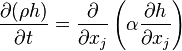(7)

.

$h$ is the specific enthalpy, $\rho$ the density and $\alpha = \kappa / c_p$ is the thermal diffusivity which is defined as the ratio between the thermal conductivity $\kappa$ and the specific heat capacity $c_p$. Note that $\kappa$ can be also anisotropic.

The source code can be found in solveSolid.H:

 
 
{
    while (pimple.correctNonOrthogonal())
    {
        fvScalarMatrix hEqn
        (
            fvm::ddt(betav*rho, h)
          - (
                thermo.isotropic()
              ? fvm::laplacian(betav*thermo.alpha(), h, "laplacian(alpha,h)")
              : fvm::laplacian(betav*taniAlpha(), h, "laplacian(alpha,h)")
            )
          ==
            fvOptions(rho, h)
        );
 
        hEqn.relax();
 
        fvOptions.constrain(hEqn);
 
        hEqn.solve(mesh.solver(h.select(pimples.finalIter())));
 
        fvOptions.correct(h);
    
 
thermo.correct();
 
Info<< "Min/max T:" << min(thermo.T()).value() << ' '
    << max(thermo.T()).value() << endl;
 
 

1.3 Coupling between Fluid and Solid

A good explanation of the coupling between fluid and solid can be found in https://www.cfd-online.com/Forums/openfoam-solving/143571-understanding-temperature-coupling-bcs.html.

At the interface between solid s and fluid f the temperature T for both phases that to be the same:

$T_f = T_s$

(8)

.

Furthermore the heat flux entering one region at one side of the interphase should be equal to the heat flux leaving the other region on the other side of the domain:

$Q_f = -Q_s$

(9)

.

If we neglect radiation the above expression can be written as:

$\kappa_f \frac{d T_f}{ d n} = - \kappa_s \frac{d T_s}{ d n}$

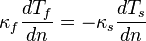(10)

.

$n$ represents the direction normal to the wall. $\kappa_f$ and $\kappa_s$ are the thermal conductivity of the fluid and solid, respectively.

The source code of the above boundary condition can be found in src/TurbulenceModels/compressible/turbulentFluidThermoModels/derivedFvPatchFields/turbulentTemperatureCoupledBaffleMixed/turbulentTemperatureCoupledBaffleMixedFvPatchScalarField.C

 
 
 
void turbulentTemperatureCoupledBaffleMixedFvPatchScalarField::updateCoeffs()
 {
     if (updated())
     {
         return;
     }
 
     // Since we're inside initEvaluate/evaluate there might be processor
     // comms underway. Change the tag we use.
     int oldTag = UPstream::msgType();
     UPstream::msgType() = oldTag+1;
 
     // Get the coupling information from the mappedPatchBase
     const mappedPatchBase& mpp =
         refCast<const mappedPatchBase>(patch().patch());
     const polyMesh& nbrMesh = mpp.sampleMesh();
     const label samplePatchi = mpp.samplePolyPatch().index();
     const fvPatch& nbrPatch =
         refCast<const fvMesh>(nbrMesh).boundary()[samplePatchi];
 
     // Calculate the temperature by harmonic averaging
     // ~~~~~~~~~~~~~~~~~~~~~~~~~~~~~~~~~~~~~~~~~~~~~~~
 
     const turbulentTemperatureCoupledBaffleMixedFvPatchScalarField& nbrField =
     refCast
     <
         const turbulentTemperatureCoupledBaffleMixedFvPatchScalarField
     >
     (
         nbrPatch.lookupPatchField<volScalarField, scalar>
         (
             TnbrName_
         )
     );
 
     // Swap to obtain full local values of neighbour internal field
     tmp<scalarField> nbrIntFld(new scalarField(nbrField.size(), 0.0));
     tmp<scalarField> nbrKDelta(new scalarField(nbrField.size(), 0.0));
 
     if (contactRes_ == 0.0)
     {
         nbrIntFld.ref() = nbrField.patchInternalField();
         nbrKDelta.ref() = nbrField.kappa(nbrField)*nbrPatch.deltaCoeffs();
     }
     else
     {
         nbrIntFld.ref() = nbrField;
         nbrKDelta.ref() = contactRes_;
     }
 
     mpp.distribute(nbrIntFld.ref());
     mpp.distribute(nbrKDelta.ref());
 
     tmp<scalarField> myKDelta = kappa(*this)*patch().deltaCoeffs();
 
 
     // Both sides agree on
     // - temperature : (myKDelta*fld + nbrKDelta*nbrFld)/(myKDelta+nbrKDelta)
     // - gradient    : (temperature-fld)*delta
     // We've got a degree of freedom in how to implement this in a mixed bc.
     // (what gradient, what fixedValue and mixing coefficient)
     // Two reasonable choices:
     // 1. specify above temperature on one side (preferentially the high side)
     //    and above gradient on the other. So this will switch between pure
     //    fixedvalue and pure fixedgradient
     // 2. specify gradient and temperature such that the equations are the
     //    same on both sides. This leads to the choice of
     //    - refGradient = zero gradient
     //    - refValue = neighbour value
     //    - mixFraction = nbrKDelta / (nbrKDelta + myKDelta())
 
     this->refValue() = nbrIntFld();
     this->refGrad() = 0.0;
     this->valueFraction() = nbrKDelta()/(nbrKDelta() + myKDelta());
 
     mixedFvPatchScalarField::updateCoeffs();
 
     if (debug)
     {
         scalar Q = gSum(kappa(*this)*patch().magSf()*snGrad());
 
         Info<< patch().boundaryMesh().mesh().name() << ':'
             << patch().name() << ':'
             << this->internalField().name() << " <- "
             << nbrMesh.name() << ':'
             << nbrPatch.name() << ':'
             << this->internalField().name() << " :"
             << " heat transfer rate:" << Q
             << " walltemperature "
             << " min:" << gMin(*this)
             << " max:" << gMax(*this)
             << " avg:" << gAverage(*this)
             << endl;
     }
 
     // Restore tag
     UPstream::msgType() = oldTag;
 }