Difference between revisions of "FireFoam"
(→Equations Fluid) |
(→Equations Fluid) |
||
| Line 560: | Line 560: | ||
===Equations Fluid=== | ===Equations Fluid=== | ||
| + | |||
| + | ====Mass conservation==== | ||
| + | |||
| + | The variable-density continuity equation is | ||
| + | |||
| + | <table width="70%"><tr><td> | ||
| + | <center><math> | ||
| + | |||
| + | \frac{\partial \rho}{\partial t} + \frac{\partial {\rho u}_j}{\partial x_j} = S_{\delta,eva} + S_{p,eva} | ||
| + | |||
| + | </math></center> | ||
| + | </td><td width="5%">(1)</td></tr></table> | ||
| + | |||
| + | |||
| + | The source terms in the mass conservation equations come from the evaporation of the liquid film <math> S_{\delta,eva} </math> and from | ||
| + | the liquid droplets <math> S_{p,eva} </math>. | ||
| + | |||
| + | The source code can be found in rhoEqn.H: | ||
| + | |||
| + | <br><cpp> | ||
| + | |||
| + | { | ||
| + | fvScalarMatrix rhoEqn | ||
| + | ( | ||
| + | fvm::ddt(rho) | ||
| + | + fvc::div(phi) | ||
| + | == | ||
| + | parcels.Srho(rho) | ||
| + | + surfaceFilm.Srho() | ||
| + | + fvOptions(rho) | ||
| + | ); | ||
| + | |||
| + | rhoEqn.solve(); | ||
| + | |||
| + | fvOptions.correct(rho); | ||
| + | } | ||
| + | |||
| + | </cpp><br> | ||
====Momentum conservation==== | ====Momentum conservation==== | ||
Revision as of 10:25, 23 April 2019
fireFoam
   Transient solver for fires and turbulent diffusion flames with reacting
   particle clouds, surface film and pyrolysis modelling.
Contents
1 Solution Strategy
The source code can be found in fireFoam.C
/*---------------------------------------------------------------------------*\
  =========                 |
  \\      /  F ield         | OpenFOAM: The Open Source CFD Toolbox
   \\    /   O peration     |
    \\  /    A nd           | Copyright (C) 2011-2017 OpenFOAM Foundation
     \\/     M anipulation  |
-------------------------------------------------------------------------------
License
    This file is part of OpenFOAM.

    OpenFOAM is free software: you can redistribute it and/or modify it
    under the terms of the GNU General Public License as published by
    the Free Software Foundation, either version 3 of the License, or
    (at your option) any later version.

    OpenFOAM is distributed in the hope that it will be useful, but WITHOUT
    ANY WARRANTY; without even the implied warranty of MERCHANTABILITY or
    FITNESS FOR A PARTICULAR PURPOSE.  See the GNU General Public License
    for more details.

    You should have received a copy of the GNU General Public License
    along with OpenFOAM.  If not, see <http://www.gnu.org/licenses/>.

Application
    fireFoam

Group
    grpCombustionSolvers

Description
    Transient solver for fires and turbulent diffusion flames with reacting
    particle clouds, surface film and pyrolysis modelling.

\*---------------------------------------------------------------------------*/

#include "fvCFD.H"
#include "turbulentFluidThermoModel.H"
#include "basicReactingCloud.H"
#include "surfaceFilmModel.H"
#include "pyrolysisModelCollection.H"
#include "radiationModel.H"
#include "SLGThermo.H"
#include "solidChemistryModel.H"
#include "psiReactionThermo.H"
#include "CombustionModel.H"
#include "pimpleControl.H"
#include "fvOptions.H"

// * * * * * * * * * * * * * * * * * * * * * * * * * * * * * * * * * * * * * //

int main(int argc, char *argv[])
{
    argList::addNote
    (
        "Transient solver for fires and turbulent diffusion flames"
        " with reacting particle clouds, surface film and pyrolysis modelling."
    );

    #include "postProcess.H"

    #include "addCheckCaseOptions.H"
    #include "setRootCaseLists.H"
    #include "createTime.H"
    #include "createMesh.H"
    #include "createControl.H"
    #include "createFields.H"
    #include "createFieldRefs.H"
    #include "initContinuityErrs.H"
    #include "createTimeControls.H"
    #include "compressibleCourantNo.H"
    #include "setInitialDeltaT.H"
    #include "createRegionControls.H"

    turbulence->validate();

    // * * * * * * * * * * * * * * * * * * * * * * * * * * * * * * * * * * * //

    Info<< "\nStarting time loop\n" << endl;

    while (runTime.run())
    {
        #include "readTimeControls.H"
        #include "compressibleCourantNo.H"
        #include "solidRegionDiffusionNo.H"
        #include "setMultiRegionDeltaT.H"
        #include "setDeltaT.H"

        ++runTime;

        Info<< "Time = " << runTime.timeName() << nl << endl;

        parcels.evolve();

        surfaceFilm.evolve();

        if(solvePyrolysisRegion)
        {
            pyrolysis.evolve();
        }

        if (solvePrimaryRegion)
        {
            #include "rhoEqn.H"

            // --- PIMPLE loop
            while (pimple.loop())
            {
                #include "UEqn.H"
                #include "YEEqn.H"

                // --- Pressure corrector loop
                while (pimple.correct())
                {
                    #include "pEqn.H"
                }

                if (pimple.turbCorr())
                {
                    turbulence->correct();
                }
            }

            rho = thermo.rho();
        }

        runTime.write();

        runTime.printExecutionTime(Info);
    }

    Info<< "End" << endl;

    return 0;
}


// ************************************************************************* //
2 Equations
2.1 Equations Liquid Film
The equation describing the evolution of the liquid film can be found in http://www.ilasseurope.org/ICLASS/iclass2012_Heidelberg/Contributions/Paper-pdfs/Contribution1294_b.pdf and https://www.witpress.com/Secure/elibrary/papers/MPF11/MPF11020FU1.pdf. A description of the method used to derive the equation can be found in https://www.researchgate.net/profile/Petr_Vita/publication/313655371_Thin_Film_Fluid_Flow_Simulation_on_Rotating_Discs/links/58a1a592a6fdccf5e9707665/Thin-Film-Fluid-Flow-Simulation-on-Rotating-Discs.pdf.
2.1.1 Mass Conservation Film
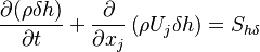
The conservation of mass reads:
 | (1) |
 represents the mean film velocity,
  the film height and
 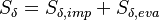 the mass source term resulting
from the impingement of the liquid droplets on the film surface
the mass source term resulting
from the impingement of the liquid droplets on the film surface  and due to the evaporation of the film
  . Note
that the source term due to evaporation will be inserted into the pressure equation for the gas phase and also into the equation for the spices
transport.
The source code of the continuity equation can be found in src/regionModels/surfaceFilmModels/kinematicSingleLayer:
. Note
that the source term due to evaporation will be inserted into the pressure equation for the gas phase and also into the equation for the spices
transport.
The source code of the continuity equation can be found in src/regionModels/surfaceFilmModels/kinematicSingleLayer:
void kinematicSingleLayer::solveContinuity()
{
    if (debug)
    {
        InfoInFunction << endl;
    }

    solve
    (
        fvm::ddt(deltaRho_)
      + fvc::div(phi_)
     ==
      - rhoSp_
    );
}
2.1.2 Momentum Conservation Film
The momentum conservation reads:
 | (2) |
 represents the pressure,
  the stress like components of the forces acting on the filme and
  represents the contribution to the momentum by the impinging droplets. The pressure contribution is divided in three components: The contribution due to capillary effects
 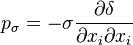 , the hydrostatic contribution
 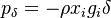 and the contribution of the pressure originated by the surrounding gas
  .
.  represents the surface tension. The stress like contribution is divided in the wall shear stress
 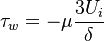 , the gravity force tangential to the wall
  and the contribution of the contact line force
  .
.  is the component of the gravity parallel to the wall. Finally the momentum equation can be written as:
 | (3) |
The source code of the momentum equation can be found in src/regionModels/surfaceFilmModels/kinematicSingleLayer:
tmp<Foam::fvVectorMatrix> kinematicSingleLayer::solveMomentum
(
    const volScalarField& pu,
    const volScalarField& pp
)
{
    if (debug)
    {
        InfoInFunction << endl;
    }

    // Momentum
    tmp<fvVectorMatrix> tUEqn
    (
        fvm::ddt(deltaRho_, U_)
      + fvm::div(phi_, U_)
     ==
      - USp_
   // - fvm::SuSp(rhoSp_, U_)
      - rhoSp_*U_
      + forces_.correct(U_)
      + turbulence_->Su(U_)
    );

    fvVectorMatrix& UEqn = tUEqn.ref();

    UEqn.relax();

    if (momentumPredictor_)
    {
        solve
        (
            UEqn
         ==
            fvc::reconstruct
            (
              - fvc::interpolate(delta_)
              * (
                    regionMesh().magSf()
                  * (
                        fvc::snGrad(pu, "snGrad(p)")
                      + fvc::snGrad(pp, "snGrad(p)")*fvc::interpolate(delta_)
                      + fvc::snGrad(delta_)*fvc::interpolate(pp)
                    )
                  - fvc::flux(rho_*gTan())
                )
            )
        );

        // Remove any patch-normal components of velocity
        U_ -= nHat()*(nHat() & U_);
        U_.correctBoundaryConditions();
    }

    return tUEqn;
}
2.1.3 Energy Conservation Film
The energy equation reads:
 | (4) |
 represents the mean film enthalpy and
  represents the contribution of the impinging droplets
  and the evaporation of the film
  to the
energy equation. Note that the energy required by the film (or a portion of it) to evaporate is cast as source term into the energy equation of the surrounding gas. The source code can be found in src/regionModels/surfaceFilmModels/thermoSingleLayer:
to the
energy equation. Note that the energy required by the film (or a portion of it) to evaporate is cast as source term into the energy equation of the surrounding gas. The source code can be found in src/regionModels/surfaceFilmModels/thermoSingleLayer:
void thermoSingleLayer::solveEnergy()
{
    if (debug)
    {
        InfoInFunction << endl;
    }


    dimensionedScalar residualDeltaRho
    (
        "residualDeltaRho",
        deltaRho_.dimensions(),
        1e-10
    );

    solve
    (
        fvm::ddt(deltaRho_, hs_)
      + fvm::div(phi_, hs_)
     ==
      - hsSp_
      + q(hs_)
      + radiation_->Shs()
    );

    correctThermoFields();

    // Evaluate viscosity from user-model
    viscosity_->correct(pPrimary_, T_);

    // Update film wall and surface temperatures
    updateSurfaceTemperatures();
}
2.1.4 Film Thickness Equation
The last equation missing is the linear equation used to get the film thickness . In order to get a tighter coupling between the momentum equation and the continuity equation, the same strategy used to get a coupling between momentum and continuity equation in pressure based solvers (see https://openfoamwiki.net/index.php/ChtMultiRegionFoam and https://openfoamwiki.net/index.php/SimpleFoam and references therein ) is used: The discrete momentum equation is used to get a relation for
the velocity at point P  which is then inserted into the continuity equation (1). The most convenient way to illustrate the procedure, is to write down the momentum equation in its discrete form:
![\rho \bold {U_p} \delta = \rho \left [ \bold { H[U] } \bold {\frac {1}{A_P}} - \bold {\frac {1}{A_P}}\delta \nabla \left ( \underbrace{-\rho g_i x_i}_{P_p} \delta - \underbrace{\sigma \nabla \nabla \delta + p_g}_{P_u} \right ) + \bold {\frac {1}{A_P}}\rho \delta g_t \right ] \delta](/images/math/1/4/4/1449081c4710027a4a917a67b76e63d8.png) | (5) |
The operator ![\bold H[U]](/images/math/a/6/5/a6568548bfa99b87e4cb0a03afad872b.png) contained the contribution of the of the neighbouring velocities and the source term to the velocity at cell centre P. The explicit and implicite source terms included into the are the contributions due to the viscose shear, the influence of the contact angle and the contribution of the
particle impingement. In order that equation (5) can be inserted into the continuity equation the divergence has to be taken:
contained the contribution of the of the neighbouring velocities and the source term to the velocity at cell centre P. The explicit and implicite source terms included into the are the contributions due to the viscose shear, the influence of the contact angle and the contribution of the
particle impingement. In order that equation (5) can be inserted into the continuity equation the divergence has to be taken:
![\rho \nabla \cdot \left ( \bold {U_p} \delta \right ) =
\rho \nabla \cdot \left ( \left [ \bold {\frac { \bold { H[U] }}{A_P}} - \bold {\frac {\delta}{A_P}} \nabla \left ( {P_p} \delta +{P_u} \right ) + {\frac {\delta}{\bold A_P}}\rho g_t \right ] \delta \right )](/images/math/d/0/1/d01b1ab158ed586aad40b8a661609dd0.png) | (6) |
The above equation can be inserted into the continuity equation to obtain:
![\frac{ \partial (\rho \delta )}{\partial t} +
\rho \nabla \cdot \left ( \left [ \bold {\frac { \bold { H[U] }}{A_P}} - \frac {\delta^2}{A_P} \nabla {P_p} - \frac {\delta P_p}{A_P} \nabla {\delta} - \bold {\frac {\delta}{A_P}} \nabla {P_u} + {\frac {\delta}{\bold A_P}}\rho g_t \right ] \delta \right ) = S_{\delta}](/images/math/a/7/5/a75cca6b4eadbbd675d0306542636176.png) | (7) |
It is obvious that the above equation is non linear in . In order to be solved it has to be linearised and an iterative method has be applied to obtain an
approximate solution.
In order to obtain the final set of equations which are solved in this solver, a Picard or fixed point iteration is used (see e.g. https://hplgit.github.io/num-methods-for-PDEs/doc/pub/nonlin/pdf/nonlin-4print.pdf or http://web.engr.uky.edu/~acfd/me690-lctr-nts.pdf):
![\frac{ \partial (\rho \delta^{k+1} )}{\partial t} +
\rho \nabla \cdot \left ( \left [ \bold {\frac { \bold { H[U] }}{A_P}} - \frac {{\delta^k}^2}{A_P} \nabla {P_p} - \frac {\delta^k P_p}{A_P} \nabla {\delta^{k+1}} - \frac {\delta^k}{\bold A_P} \nabla {P_u} + {\frac {\delta^k}{\bold A_P}}\rho g_t \right ] \delta^{k+1} \right ) = S_{\delta}](/images/math/5/4/f/54f1c220c3827744789ebcd9820f8f4b.png) | (8) |
The superscript k denote the solution computed at the last iteration an the superscript k+1 denotes the solution of the current iteration which has to be computed by solving the linear system resulting from the discretization. After separating the linear and the still non linear terms of the above equation we obtain:
![\frac{ \partial (\rho \delta^{k+1} )}{\partial t} +
\rho \nabla \cdot \left ( \left [ \bold {\frac { \bold { H[U] }}{A_P}} - \frac {{\delta^k}^2}{A_P} \nabla {P_p} - \frac {\delta^k}{\bold A_P} \nabla {P_u} + {\frac {\delta^k}{\bold A_P}}\rho g_t \right ] \delta^{k+1} \right ) - \nabla \cdot \left ( \frac {\delta^k\delta^{k+1} P_p}{A_P} \nabla {\delta^{k+1}} \right ) = S_{\delta}](/images/math/8/2/3/823a63f544781d33fd0bacc9b5ba0531.png) | (9) |
Since the above equation still contains a non linear contribution it has remaining  has to be approximated by the value at the previous iteration step
 :
:
![\frac{ \partial (\rho \delta^{k+1} )}{\partial t} +
\rho \nabla \cdot \left ( \left [ \bold {\frac { \bold { H[U] }}{A_P}} - \frac {{\delta^k}^2}{A_P} \nabla {P_p} - \frac {\delta^k}{\bold A_P} \nabla {P_u} + {\frac {\delta^k}{\bold A_P}}\rho g_t \right ] \delta^{k+1} \right ) - \nabla \cdot \left ( \frac {\delta^k\delta^{k} P_p}{A_P} \nabla {\delta^{k+1}} \right ) = S_{\delta}](/images/math/f/c/b/fcb9c168d16e87fc3f62d76c091541b5.png) | (10) |
which is the final form solved in the present solver. The source code can be found in src/regionModels/surfaceFilmModels/kinematicSingleLayer:
void kinematicSingleLayer::solveThickness
(
    const volScalarField& pu,
    const volScalarField& pp,
    const fvVectorMatrix& UEqn
)
{
    if (debug)
    {
        InfoInFunction << endl;
    }

    volScalarField rUA(1.0/UEqn.A());
    U_ = rUA*UEqn.H();

    surfaceScalarField deltarUAf(fvc::interpolate(delta_*rUA));
    surfaceScalarField rhof(fvc::interpolate(rho_));

    surfaceScalarField phiAdd
    (
        "phiAdd",
        regionMesh().magSf()
      * (
            fvc::snGrad(pu, "snGrad(p)")
          + fvc::snGrad(pp, "snGrad(p)")*fvc::interpolate(delta_)
        )
      - fvc::flux(rho_*gTan())
    );
    constrainFilmField(phiAdd, 0.0);

    surfaceScalarField phid
    (
        "phid",
        fvc::flux(U_*rho_) - deltarUAf*phiAdd*rhof
    );
    constrainFilmField(phid, 0.0);

    surfaceScalarField ddrhorUAppf
    (
        "deltaCoeff",
        fvc::interpolate(delta_)*deltarUAf*rhof*fvc::interpolate(pp)
    );

    regionMesh().setFluxRequired(delta_.name());

    for (int nonOrth=0; nonOrth<=nNonOrthCorr_; nonOrth++)
    {
        // Film thickness equation
        fvScalarMatrix deltaEqn
        (
            fvm::ddt(rho_, delta_)
          + fvm::div(phid, delta_)
          - fvm::laplacian(ddrhorUAppf, delta_)
         ==
          - rhoSp_
        );

        deltaEqn.solve();

        if (nonOrth == nNonOrthCorr_)
        {
            phiAdd +=
                fvc::interpolate(pp)
              * fvc::snGrad(delta_)
              * regionMesh().magSf();

            phi_ == deltaEqn.flux();
        }
    }

    // Bound film thickness by a minimum of zero
    delta_.max(0.0);

    // Update U field
    U_ -= fvc::reconstruct(deltarUAf*phiAdd);

    // Remove any patch-normal components of velocity
    U_ -= nHat()*(nHat() & U_);

    U_.correctBoundaryConditions();

    // Update film wall and surface velocities
    updateSurfaceVelocities();

    // Continuity check
    continuityCheck();
}
2.1.5 Solution Strategy
Equations (1), (3) and (4) represent a system of 3 non-linear partial differential equations with the unknowns ,  and . In order to solve this system of equations, a splitting method is adopted: The equations are linearised by using quantities from the previous iteration and solved sequentially. The steps performed are the following:
1. Solve continuity equation (1). Here has to be mentioned that the quantity solved for is  which appears also in the momentum and energy equation.
2. Solve momentum equation (3)
3. Solve energy equation (4)
4. Solve film thickness equation: The film thickness equation is derived by inserting the discrete momentum equation into the continuity equation.
Steps 2-4 are solved a number of time specified by the user in order to achieve sufficient convergence of the equations. The source code can be found in src/regionModels/surfaceFilmModels/thermoSingleLayer
 void thermoSingleLayer::evolveRegion()
{
    if (debug)
    {
        InfoInFunction << endl;
    }

    // Solve continuity for deltaRho_
    solveContinuity();

    // Update sub-models to provide updated source contributions
    updateSubmodels();

    // Solve continuity for deltaRho_
    solveContinuity();

    for (int oCorr=1; oCorr<=nOuterCorr_; oCorr++)
    {
        // Explicit pressure source contribution
        tmp<volScalarField> tpu(this->pu());

        // Implicit pressure source coefficient
        tmp<volScalarField> tpp(this->pp());

        // Solve for momentum for U_
        tmp<fvVectorMatrix> UEqn = solveMomentum(tpu(), tpp());

        // Solve energy for hs_ - also updates thermo
        solveEnergy();

        // Film thickness correction loop
        for (int corr=1; corr<=nCorr_; corr++)
        {
            // Solve thickness for delta_
            solveThickness(tpu(), tpp(), UEqn());
        }
    }

    // Update deltaRho_ with new delta_
    deltaRho_ == delta_*rho_;

    // Update temperature using latest hs_
    T_ == T(hs_);
}
2.2 Equations Fluid
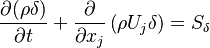
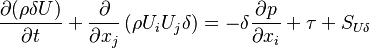
2.2.1 Mass conservation
The variable-density continuity equation is
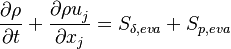 | (1) |
The source terms in the mass conservation equations come from the evaporation of the liquid film and from
the liquid droplets  .
.
The source code can be found in rhoEqn.H:
{
    fvScalarMatrix rhoEqn
    (
        fvm::ddt(rho)
      + fvc::div(phi)
      ==
        parcels.Srho(rho)
      + surfaceFilm.Srho()
      + fvOptions(rho)
    );

    rhoEqn.solve();

    fvOptions.correct(rho);
}
2.2.2 Momentum conservation
The equation of motion are written for a moving frame of reference. They are however formulated for the absolute velocity (the derivation of the equations of motion can be found in https://openfoamwiki.net/index.php/See_the_MRF_development and also in https://diglib.tugraz.at/download.php?id=581303c7c91f9&location=browse. Some additional information can be found in https://pingpong.chalmers.se/public/pp/public_courses/course07056/published/1497955220499/resourceId/3711490/content/UploadedResources/HakanNilssonRotatingMachineryTrainingOFW11-1.pdf):
 | (2) |
 represent the velocity,
  the relative veloicty,
  the gravitational acceleration,
 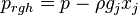 the pressure minus the hydrostatic pressure and
 and
and  are the viscose and turbulent stresses. Note that since the relative velocity appears in the divergence term, the
face flux
are the viscose and turbulent stresses. Note that since the relative velocity appears in the divergence term, the
face flux  appearing in the finite volume discretization of the momentum equation should be calculated with the relative velocity.
 represents the force excreted by the particles on the fluid.
The source code can be found in Ueqn.H:
      MRF.correctBoundaryVelocity(U);

    fvVectorMatrix UEqn
    (
        fvm::ddt(rho, U) + fvm::div(phi, U)
      + MRF.DDt(rho, U)
      + turbulence->divDevRhoReff(U)
     ==
        parcels.SU(U)
      + fvOptions(rho, U)
    );

    UEqn.relax();

    fvOptions.constrain(UEqn);

    if (pimple.momentumPredictor())
    {
        solve
        (
            UEqn
          ==
            fvc::reconstruct
            (
                (
                  - ghf*fvc::snGrad(rho)
                  - fvc::snGrad(p_rgh)
                )*mesh.magSf()
            )
        );

        fvOptions.correct(U);
        K = 0.5*magSqr(U);
    }
2.2.3 Species conservation
In order to account for the chemical reactions occurring between different chemical species a conservation equation for each species k has to be solved:
 | (6) |
 is the reaction rate of the species k and
 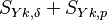 is the contribution to the spices k by the evaporation of the film and the particle respectively.
The source code can be found in YEEqn.H:
tmp<fv::convectionScheme<scalar>> mvConvection
(
    fv::convectionScheme<scalar>::New
    (
        mesh,
        fields,
        phi,
        mesh.divScheme("div(phi,Yi_h)")
    )
);
{
    combustion->correct();
    Qdot = combustion->Qdot();
    volScalarField Yt(0.0*Y[0]);

    forAll(Y, i)
    {
        if (i != inertIndex && composition.active(i))
        {
            volScalarField& Yi = Y[i];

            fvScalarMatrix YiEqn
            (
                fvm::ddt(rho, Yi)
              + mvConvection->fvmDiv(phi, Yi)
              - fvm::laplacian(turbulence->alphaEff(), Yi)
              ==
                parcels.SYi(i, Yi)
              + surfaceFilm.Srho(i)
              + combustion->R(Yi)
              + fvOptions(rho, Yi)
            );

            YiEqn.relax();

            fvOptions.constrain(YiEqn);

            YiEqn.solve(mesh.solver("Yi"));

            fvOptions.correct(Yi);

            Yi.max(0.0);
            Yt += Yi;
        }
    }

    Y[inertIndex] = scalar(1) - Yt;
    Y[inertIndex].max(0.0);

    radiation->correct();
2.2.4 Energy conservation
The derivation of the energy equation (without source terms from the evaporation of the particle  and the liquid film ) can be found in: https://cfd.direct/openfoam/energy-equation/
The total energy of a fluid element can be seen as the sum of kinetic energy  and internal energy
  .
The rate of change of the kinetic energy within a fluid element is the work done on this fluid element by the viscous forces, the pressure and eternal volume forces like the gravity:
.
The rate of change of the kinetic energy within a fluid element is the work done on this fluid element by the viscous forces, the pressure and eternal volume forces like the gravity:
 | (3) |
The rate of change of the internal energy of a fluid element is the heat transferred to this fluid element by diffusion and turbulence  plus the
heat source term
plus the
heat source term  plus the heat source by radiation
  :
:
 | (4) |
The change rate of the total energy is the sum of the above two equations:
 | (5) |
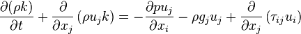
Instead of the internal energy there is also the option to solve the equation for the enthalpy 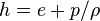 :
:
 | (5) |
The source code can be found in YEEqn.H:
    volScalarField& he = thermo.he();

    fvScalarMatrix EEqn
    (
        fvm::ddt(rho, he) + mvConvection->fvmDiv(phi, he)
      + fvc::ddt(rho, K) + fvc::div(phi, K)
      + (
            he.name() == "e"
          ? fvc::div
            (
                fvc::absolute(phi/fvc::interpolate(rho), U),
                p,
                "div(phiv,p)"
            )
          : -dpdt
        )
      - fvm::laplacian(turbulence->alphaEff(), he)
     ==
        Qdot
      + radiation->Sh(thermo, he)
      + parcels.Sh(he)
      + surfaceFilm.Sh()
      + fvOptions(rho, he)
    );

    EEqn.relax();

    fvOptions.constrain(EEqn);

    EEqn.solve();

    fvOptions.correct(he);

    thermo.correct();

    Info<< "min/max(T) = "
        << min(T).value() << ", " << max(T).value() << endl;