Difference between revisions of "HowTo post-process multiphase results"
From OpenFOAMWiki
(Kick off this page. Will continue in a few minutes) |
m (Added to the category ParaFoam) |
||
| (5 intermediate revisions by 2 users not shown) | |||
| Line 1: | Line 1: | ||
= Introduction = | = Introduction = | ||
| − | OpenFOAM handles multiphase simulations with the [[interFoam]] solvers through using a single field that represents the phase present at a certain cell, face or vertex. The field is usually named {{tt|alpha}} or {{tt|alpha1}}. | + | OpenFOAM handles multiphase simulations with the [[interFoam]] type solvers through using a single field that represents the phase present at a certain cell, face or vertex. The field is usually named {{tt|alpha}} or {{tt|alpha1}}. |
Therefore, given that it's a single field, this means that: | Therefore, given that it's a single field, this means that: | ||
| Line 21: | Line 21: | ||
</li> | </li> | ||
| − | <li> | + | <li>As shown in the [[#Figure_1|Figure 1]], select the fields {{tt|alpha1}} and {{tt|p_rgh}} on the lower left and then click on the {{tt|Apply}} button on the left. |
| + | [[Image:HowTo post-process multiphase results 00.png|thumb|450px|center|<div id="Figure_1">Figure 1: This example is using the {{tt|damBreak}} tutorial. Choose the fields and apply.</div>]] | ||
</li> | </li> | ||
| − | <li> | + | <li>On [[#Figure_2|Figure 2]] is shown where to switch to wireframe representation, as well as showing the {{tt|alpha1}} field. As for turning on the colour legend, it's the button on the left. |
| − | + | ||
| − | < | + | [[Image:HowTo post-process multiphase results 01.png|thumb|450px|center|<div id="Figure_2">Figure 2: Pick to see the {{tt|alpha1}} field, in {{tt|wireframe}} mode and choose to see the colour legend.</div>]] |
</li> | </li> | ||
| − | <li> | + | <li>On [[#Figure_3|Figure 3]] is shown where to looks at for applying the contour isosurface and respective configurations, starting from the button on the top right, then down to the left to select the field for the contour and the values for which to show isosurfaces. Don't forget to click on the {{tt|Apply button}} to activate the contour filter. |
| − | + | ||
| − | < | + | [[Image:HowTo post-process multiphase results 02.png|thumb|450px|center|<div id="Figure_3">Figure 3: Apply the {{tt|Contour}} filter and choose to represent the {{tt|alpha1}} field with a single isosurface at the value {{tt|0.5}}.</div>]] |
</li> | </li> | ||
| − | <li> | + | <li>In order to change the current time instance to be represented, have a look at [[#Figure_4|Figure 4]]. The number {{tt|20}} indicates that it's the 20th time instance, indexed to zero; in other words, it's the 21st time instance, if the very first 0 time is counted. |
| − | + | ||
| − | < | + | [[Image:HowTo post-process multiphase results 03.png|thumb|450px|center|<div id="Figure_4">Figure 4: Skip ahead in time and change the camera perspective to see better the isosurface between the two phases.</div>]] |
</li> | </li> | ||
| − | <li> | + | <li>On [[#Figure_5|Figure 5]] demonstrated how to see the outline of the mesh (namely the bounding box, not the feature edges), so that it's clearer to see the isosurface. |
| + | |||
| + | [[Image:HowTo post-process multiphase results 04.png|thumb|450px|center|<div id="Figure_5">Figure 5: Choose to see the outline of the mesh, to make it easier to see the isosurface.</div>]] | ||
</li> | </li> | ||
| − | <li> | + | <li>On [[#Figure_6|Figure 6]] is another tutorial example, namely the {{tt|floatingObject}}, located at {{tt|multiphase/interDyMFoam/ras/floatingObject}}. Try to figure out how to achieve this view, as already demonstrated in the first steps. |
| + | |||
| + | [[Image:HowTo post-process multiphase results 05.png|thumb|450px|center|<div id="Figure_6">Figure 6: Another example, now using the {{tt|floatingObject}} tutorial.</div>]] | ||
</li> | </li> | ||
| − | <li> | + | <li>Since this case has a floating box inside the domain, do as indicated on [[#Figure_7|Figure 7]], by opening the same case a second time (it's the button on the top left). Then for the newly loaded file, choose only the {{tt|floatingObject}} patch, click on the {{tt|Apply button}} and choose to see the surface. |
| + | |||
| + | [[Image:HowTo post-process multiphase results 06.png|thumb|450px|center|<div id="Figure_7">Figure 7: Open the same case twice and choose to see the surface of only the patch for the floating block.</div>]] | ||
</li> | </li> | ||
| − | <li> | + | <li>On [[#Figure_8|Figure 8]] is what the first time instance looks like (at the ''zero'' second), using the contour filter, which is applied to the first file. |
| + | |||
| + | [[Image:HowTo post-process multiphase results 07.png|thumb|450px|center|<div id="Figure_8">Figure 8: Here's what it looks like when using the isosurface on the first file.</div>]] | ||
</li> | </li> | ||
| − | <li> | + | <li>On [[#Figure_9|Figure 9]] is shown another time instance at another point of view. |
| + | |||
| + | [[Image:HowTo post-process multiphase results 08.png|thumb|450px|center|<div id="Figure_9">Figure 9: What it looks like at {{tt|0.3}} s.</div>]] | ||
</li> | </li> | ||
</ol> | </ol> | ||
| − | |||
= Tips = | = Tips = | ||
* How to keep track of the height at a certain position: [http://www.cfd-online.com/Forums/paraview/112572-temporal-analysis.html#post405615 Temporal Analysis - post #2] | * How to keep track of the height at a certain position: [http://www.cfd-online.com/Forums/paraview/112572-temporal-analysis.html#post405615 Temporal Analysis - post #2] | ||
| + | |||
| + | [[Category:Tutorials]] | ||
| + | [[Category:Post-processing utilities]] | ||
| + | [[Category:Multiphase flow]] | ||
| + | [[Category:ParaFoam]] | ||
Latest revision as of 08:56, 2 November 2013
1 Introduction
OpenFOAM handles multiphase simulations with the interFoam type solvers through using a single field that represents the phase present at a certain cell, face or vertex. The field is usually named alpha or alpha1.
Therefore, given that it's a single field, this means that:
- values of 0 indicates that the phase at that cell/face/vertex is only the first phase;
- while 1 indicates that it's only the second phase.
- Anything in between is a mixture of the two phases, at a reason implied by the value.
The simplest example is 0.5, which means that it's a mix of equal proportion of the first and the second phase. In other words, this should be an indication of where the separation surface is between each phase.
- Notes
- Make sure to study well the tutorial damBreak, as explained in OpenFOAM's User Guide: 2.3 Breaking of a dam
2 Steps using paraFoam
- After running the multiphase solver, run paraFoam:
paraFoam
- As shown in the Figure 1, select the fields alpha1 and p_rgh on the lower left and then click on the Apply button on the left.
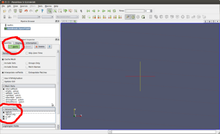
 Figure 1: This example is using the damBreak tutorial. Choose the fields and apply.
 - On Figure 2 is shown where to switch to wireframe representation, as well as showing the alpha1 field. As for turning on the colour legend, it's the button on the left.
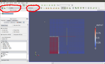 Figure 2: Pick to see the alpha1 field, in wireframe mode and choose to see the colour legend.
 - On Figure 3 is shown where to looks at for applying the contour isosurface and respective configurations, starting from the button on the top right, then down to the left to select the field for the contour and the values for which to show isosurfaces. Don't forget to click on the Apply button to activate the contour filter.
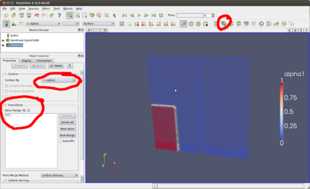 Figure 3: Apply the Contour filter and choose to represent the alpha1 field with a single isosurface at the value 0.5.
 - In order to change the current time instance to be represented, have a look at Figure 4. The number 20 indicates that it's the 20th time instance, indexed to zero; in other words, it's the 21st time instance, if the very first 0 time is counted.
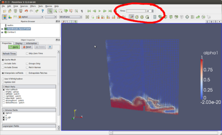 Figure 4: Skip ahead in time and change the camera perspective to see better the isosurface between the two phases.
 - On Figure 5 demonstrated how to see the outline of the mesh (namely the bounding box, not the feature edges), so that it's clearer to see the isosurface.
 Figure 5: Choose to see the outline of the mesh, to make it easier to see the isosurface.
 - On Figure 6 is another tutorial example, namely the floatingObject, located at multiphase/interDyMFoam/ras/floatingObject. Try to figure out how to achieve this view, as already demonstrated in the first steps.
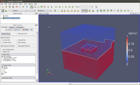 Figure 6: Another example, now using the floatingObject tutorial.
 - Since this case has a floating box inside the domain, do as indicated on Figure 7, by opening the same case a second time (it's the button on the top left). Then for the newly loaded file, choose only the floatingObject patch, click on the Apply button and choose to see the surface.
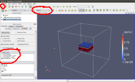 Figure 7: Open the same case twice and choose to see the surface of only the patch for the floating block.
 - On Figure 8 is what the first time instance looks like (at the zero second), using the contour filter, which is applied to the first file.
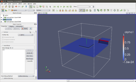 Figure 8: Here's what it looks like when using the isosurface on the first file.
 - On Figure 9 is shown another time instance at another point of view.
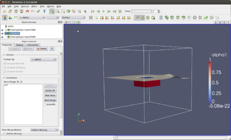 Figure 9: What it looks like at 0.3 s.


3 Tips
- How to keep track of the height at a certain position: Temporal Analysis - post #2