HowTo post-process multiphase results

1 Introduction

OpenFOAM handles multiphase simulations with the interFoam solvers through using a single field that represents the phase present at a certain cell, face or vertex. The field is usually named alpha or alpha1.

Therefore, given that it's a single field, this means that:

1. values of 0 indicates that the phase at that cell/face/vertex is only the first phase;
2. while 1 indicates that it's only the second phase.
3. Anything in between is a mixture of the two phases, at a reason implied by the value.

The simplest example is 0.5, which means that it's a mix of equal proportion of the first and the second phase. In other words, this should be an indication of where the separation surface is between each phase.

Notes

• Make sure to study well the tutorial damBreak, as explained in OpenFOAM's User Guide: 2.3 Breaking of a dam

2 Steps using paraFoam

1. After running the multiphase solver, run paraFoam:

   paraFoam

2. As shown in the Figure 1, select the fields alpha1 and p_rgh on the lower left and then click on the Apply button on the left.
   

   

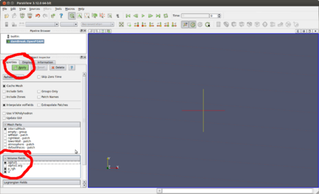
   Figure 1: This example is using the damBreak tutorial. Choose the fields and apply.
3. On Figure 2 is shown how you can see...
   

   

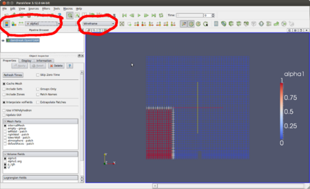   Figure 2: Pick to see the alpha1 field, in wireframe mode and choose to see the colour legend.
4. Figure 3
   

   

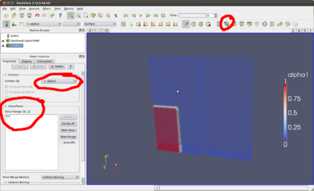   Figure 3: Apply the Contour filter and choose to represent the alpha1 field with a single isosurface at the value 0.5.
5. Figure 4
   

   

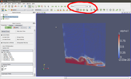   Figure 4: Skip ahead in time and change the camera perspective to see better the isosurface between the two phases.
6. Figure 5
   

   

   Figure 5: Choose to see the outline of the geometry, to make it easier to see the isosurface.
7. Figure 6
   

   

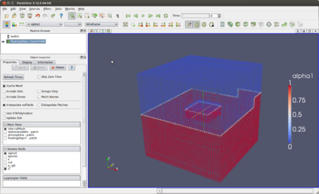   Figure 6: Another example, now using the floatingObject tutorial.
8. Figure 7
   

   

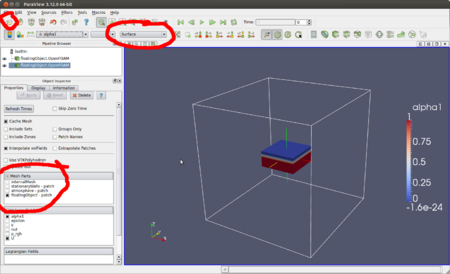   Figure 7: Open the same case twice and choose to see the surface of only the patch for the floating block.
9. Figure 8
   

   

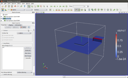   Figure 8: Here's what it looks like when using the isosurface on the first file.
10. Figure 9
    

    

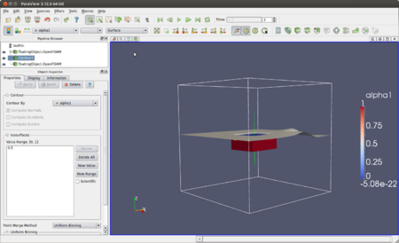    Figure 9: What it looks like at 0.3 s.

3 Tips

• How to keep track of the height at a certain position: Temporal Analysis - post #2