OpenFOAM guide/The SIMPLE algorithm in OpenFOAM

1 The Navier-Stokes equation

The Navier-Stokes equations for a single-phase flow with a constant density and viscosity are the following:

$\nabla \cdot \left( \rho \vec{U} \right) = 0$

$\frac{\partial U}{\partial t} + \nabla \cdot \left( \vec{v} \vec{v} \right) - \nabla \cdot \left( \nu \nabla \vec{v} \right) = - \nabla p$

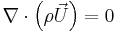
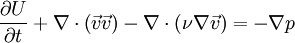
The solution of this couple of equations is not straightforward because an explicit equation for the pressure is not available. One of the most common approaches is to derive an equation for the pressure by taking the divergence of the momentum equation and by substituting it in the continuity equation.

2 The pressure equation

The momentum equation can be re-written in a semi discretised form as follows:

$a_p \vec{U_p} = H(\vec{U}) - \nabla p \Longleftrightarrow \vec{U_p} = \frac{H(\vec{U})}{a_p} - \frac{\nabla p}{a_p}$

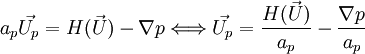
where

$H(\vec{U}) = - \sum_n a_n \vec{U}_n + \frac{\vec{U}^o}{\Delta t}$

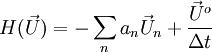
The first term of $H(\vec{U})$ represents the matrix coefficients of the neighbouring cells multiplied by their velocity, while the second part contains the unsteady term and all the sources except the pressure gradient.

The continuity equation is discretised as:

$\nabla \cdot \vec{U} = \sum_f \vec{S} \vec{U}_f$

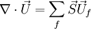
where $\vec{S}$ is outward-pointing face area vector and $\vec{U}_f$ the velocity on the face.

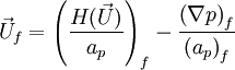
The velocity on the face is obtained by interpolating the semi discretised form of the momentum equation as follows:

$\vec{U}_f = \left( \frac{H(\vec{U})}{a_p}\right)_f - \frac{\left( \nabla p\right)_f }{\left( a_p\right)_f}$

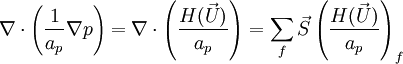
By substituting this equation into the discretised continuity equation obtained above, we obtain the pressure equation:

$\nabla \cdot \left( \frac{1}{a_p} \nabla p \right) = \nabla \cdot \left( \frac{H(\vec{U})}{a_p} \right) = \sum_f \vec{S} \left( \frac{H(\vec{U})}{a_p}\right)_f$

3 Implementation of the SIMPLE algorithm in OpenFOAM

The SIMPLE algorithm can be implemented in OpenFOAM as follows (The complete implementation of the algorithm can be seen in the source code of the simpleFoam solver provided with OpenFOAM):

• Store the pressure calculated at the previous iteration, because it is required to apply under-relaxation

 
 p.storePrevIter();

• Define the equation for U

 
 tmp<fvVectorMatrix> UEqn
 (
      fvm::div(phi, U) - laplacian(nu, U)
 );

• Under-relax the equation for U

 
 UEqn.relax();

• Solve the momentum predictor

 
 solve (UEqn == -fvc::grad(p));

• Update the boundary conditions for p

 
 p.boundaryField().updateCoeffs();

• Calculate the $a_p$ coefficient and calculate U

 
 volScalarField AU = UEqn().A();
 U = UEqn().H()/AU;
 UEqn.clear();

• Calculate the flux

 
 phi = fvc::interpolate(U) & mesh.Sf();
 adjustPhi(phi, U, p);

• Define and solve the pressure equation and repeat for the prescribed number of non-orthogonal corrector steps

 
 fvScalarMatrix pEqn
 (
   fvm::laplacian(1.0/AU, p) == fvc::div(phi)
 );
 pEqn.setReference(pRefCell, pRefValue);
 pEqn.solve();

• Correct the flux

 
 phi -= pEqn.flux();

• Under-relax the pressure for the momentum corrector and apply the correction

 
 p.relax();
 U -= fvc::grad(p)/AU;
 U.correctBoundaryConditions();

• Check for convergence and repeat from the beginning until convergence criteria are satisfied.

4 References

J. H. Ferziger, M. Peric, Computational Methods for Fluid Dynamics, Springer, 3rd Ed., 2001.

H. Jasak, Error Analysis and Estimation for the Finite Volume Method with Applications to Fluid Flows, Ph.D. Thesis, Imperial College, London, 1996.