OverPimpleDyMFoam
Transient solver for incompressible flow of Newtonian fluids on a moving mesh using the PIMPLE (merged PISO-SIMPLE) algorithm. Turbulence modelling is generic, i.e. laminar, RAS or LES may be selected.
Contents
1 Solution Strategy
The solver follows a segregated solution strategy. This means that the equations for each variable characterizing the system (the velocity  , the pressure
  and the variables characterizing turbulence) is solved sequentially
and the solution of the preceding equations is inserted in the subsequent equation. The non-linearity appearing in the momentum equation (the face flux
and the variables characterizing turbulence) is solved sequentially
and the solution of the preceding equations is inserted in the subsequent equation. The non-linearity appearing in the momentum equation (the face flux
 which is a function of the velocity) is resolved by computing it from the velocity and pressure values of the preceding iteration. The dependence from
the pressure is introduced to avoid a decoupling between the momentum and pressure equations and hence the appearance of high frequency oscillation in the solution (check board effect).
The first equation to be solve is the momentum equation. It delivers a velocity field
which is a function of the velocity) is resolved by computing it from the velocity and pressure values of the preceding iteration. The dependence from
the pressure is introduced to avoid a decoupling between the momentum and pressure equations and hence the appearance of high frequency oscillation in the solution (check board effect).
The first equation to be solve is the momentum equation. It delivers a velocity field  which is in general not divergence free, i.e.
it does not satisfy the continuity equation. After that the momentum and the continuity equations are used to construct an equation for the pressure. The
aim is to obtain a pressure field
which is in general not divergence free, i.e.
it does not satisfy the continuity equation. After that the momentum and the continuity equations are used to construct an equation for the pressure. The
aim is to obtain a pressure field  , which, if inserted in the momentum equation, delivers a divergence free velocity field .
After correcting the velocity field, the equations for turbulence are solved.
The above iterative solution procedure is repeated until convergence.
, which, if inserted in the momentum equation, delivers a divergence free velocity field .
After correcting the velocity field, the equations for turbulence are solved.
The above iterative solution procedure is repeated until convergence.
The overset method allows to solve the governing equaiton on a set of disjoint meshes, i.e., the meshes are not connected over faces. The coupling between the differnt meshes is done over an implicit interpolation.
The source code can be found in overPimpleDyMFoam.C
/*---------------------------------------------------------------------------*\
  =========                 |
  \\      /  F ield         | OpenFOAM: The Open Source CFD Toolbox
   \\    /   O peration     |
    \\  /    A nd           | www.openfoam.com
     \\/     M anipulation  |
-------------------------------------------------------------------------------
    Copyright (C) 2011-2016 OpenFOAM Foundation
    Copyright (C) 2016-2018 OpenCFD Ltd.
-------------------------------------------------------------------------------
License
    This file is part of OpenFOAM.

    OpenFOAM is free software: you can redistribute it and/or modify it
    under the terms of the GNU General Public License as published by
    the Free Software Foundation, either version 3 of the License, or
    (at your option) any later version.

    OpenFOAM is distributed in the hope that it will be useful, but WITHOUT
    ANY WARRANTY; without even the implied warranty of MERCHANTABILITY or
    FITNESS FOR A PARTICULAR PURPOSE.  See the GNU General Public License
    for more details.

    You should have received a copy of the GNU General Public License
    along with OpenFOAM.  If not, see <http://www.gnu.org/licenses/>.

Application
    overPimpleDyMFoam

Group
    grpIncompressibleSolvers grpMovingMeshSolvers

Description
    Transient solver for incompressible flow of Newtonian fluids
    on a moving mesh using the PIMPLE (merged PISO-SIMPLE) algorithm.

    Turbulence modelling is generic, i.e. laminar, RAS or LES may be selected.

\*---------------------------------------------------------------------------*/

#include "fvCFD.H"
#include "dynamicFvMesh.H"
#include "singlePhaseTransportModel.H"
#include "turbulentTransportModel.H"
#include "pimpleControl.H"
#include "fvOptions.H"

#include "cellCellStencilObject.H"
#include "zeroGradientFvPatchFields.H"
#include "localMin.H"
#include "interpolationCellPoint.H"
#include "transform.H"
#include "fvMeshSubset.H"
#include "oversetAdjustPhi.H"

// * * * * * * * * * * * * * * * * * * * * * * * * * * * * * * * * * * * * * //

int main(int argc, char *argv[])
{
    argList::addNote
    (
        "Transient solver for incompressible, turbulent flow"
        " on a moving mesh."
    );

    #include "postProcess.H"

    #include "setRootCaseLists.H"
    #include "createTime.H"
    #include "createDynamicFvMesh.H"
    #include "initContinuityErrs.H"

    pimpleControl pimple(mesh);

    #include "createFields.H"
    #include "createUf.H"
    #include "createMRF.H"
    #include "createFvOptions.H"
    #include "createControls.H"
    #include "CourantNo.H"
    #include "setInitialDeltaT.H"

    turbulence->validate();

    // * * * * * * * * * * * * * * * * * * * * * * * * * * * * * * * * * * * //

    Info<< "\nStarting time loop\n" << endl;

    while (runTime.run())
    {
        #include "readControls.H"
        #include "CourantNo.H"

        #include "setDeltaT.H"

        ++runTime;

        Info<< "Time = " << runTime.timeName() << nl << endl;

        bool changed = mesh.update();

        if (changed)
        {
            #include "setCellMask.H"
            #include "setInterpolatedCells.H"

            surfaceScalarField faceMaskOld
            (
                localMin<scalar>(mesh).interpolate(cellMask.oldTime())
            );

            // Zero Uf on old faceMask (H-I)
            Uf *= faceMaskOld;
            // Update Uf and phi on new C-I faces
            Uf += (1-faceMaskOld)*fvc::interpolate(U);
            phi = mesh.Sf() & Uf;

            // Zero phi on current H-I
            surfaceScalarField faceMask
            (
                localMin<scalar>(mesh).interpolate(cellMask)
            );
            phi *= faceMask;
        }


        if (mesh.changing() && correctPhi)
        {
            // Calculate absolute flux from the mapped surface velocity
            #include "correctPhi.H"
        }

        // Make the flux relative to the mesh motion
        fvc::makeRelative(phi, U);

        if (mesh.changing() && checkMeshCourantNo)
        {
            #include "meshCourantNo.H"
        }

        // --- Pressure-velocity PIMPLE corrector loop
        while (pimple.loop())
        {
            #include "UEqn.H"

            // --- Pressure corrector loop
            while (pimple.correct())
            {
                #include "pEqn.H"
            }

            if (pimple.turbCorr())
            {
                laminarTransport.correct();
                turbulence->correct();
            }
        }

        runTime.write();

        runTime.printExecutionTime(Info);
    }

    Info<< "End\n" << endl;

    return 0;
}


// ************************************************************************* //
2 Equations
The equation of motion used for moving meshes are written in the Arbitrary-Euler-Lagrange (ALE) formulation. This formulation is one of the most popular if morphing meshes are used to describe the solid body deformation or displacement [1]. If the overset method is used, this formulation avoids to formulate the equation of motion in multiple frames of references [2]. For the derivation of the equation see [3] [4]. The continuity and momentum equation read in this form:
-
 | (1) |
-
 | (1) |
In the above equations $\U$ is the fluid velocity, the pressure,  the molecular viscosity and
  the density. The only difference to the equation of motion in a fixed mesh is the introduction of a new variable, i.e. the grid velocity
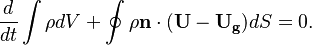
  . In order to determine the grid velocity the space conservation law (SCL) has to be solved (see also [5] [6])
-
 | (1) |
In order to not introduce additional mass conservation errors, the temporal discretisation of the SCL should be the same as used in the other conservation equation (see also [7] [8])
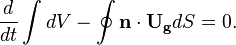
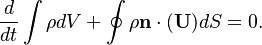
OpenFOAM uses a slightly different continuity equation (which is used to derive the equation for the pressure). By inserting the mass conservation law into the continuity equation we get for the spatial case of incompressible case:
-
 | (1) |
It is the same as the one for fixed grids. Note this transformation is valid only for incompressible flows.
2.1 Momentum Equation
In this section we will analyze the momentum equation implemented in the solver a bit more in detail. Es already seen above, the momentum equation reads:
-
 | (1) |
 is the mass flux over the surface
  .
.  is the angular velocity of the rotating frame of reference. We see that the momentum equation is essentially the same as the one in fixed control volume. See, e.g. https://openfoamwiki.net/index.php/SimpleFoam. The only difference is how the phase flux is calculated. In a fixed mesh, only the velocity in the inertial coordinate system
  is used to calculate it, while for the overset mesh the difference between the velocity in the inertial coordinate system <math< \mathbf{U} </math> and the grid velocity is used.
The source code of the momentum equation is shown above. We see that in front of the pressure equation the field cellMask is applied. It is 0 for hole cells and 1 elsewhere. This means that for background cells which are covered by a solid structure the pressure gradient term does not give any contribution to the momentum equation.
// Solve the Momentum equation

MRF.correctBoundaryVelocity(U);

tmp<fvVectorMatrix> tUEqn
(
    fvm::ddt(U) + fvm::div(phi, U)
  + MRF.DDt(U)
  + turbulence->divDevReff(U)
 ==
    fvOptions(U)
);
fvVectorMatrix& UEqn = tUEqn.ref();

UEqn.relax();

fvOptions.constrain(UEqn);

if (pimple.momentumPredictor())
{
    solve(UEqn == -cellMask*fvc::grad(p));

    fvOptions.correct(U);
}
2.2 Pressure Equation
Since the continuity equation for incompressible flow written in an AEL (arbitrary Euler-Lagrange) formulation is the same as for fixed grid (see previous section), also the pressure equation is basically the same. For this reason the derivation of the pressure equation is omitted. For a detailed derivation see https://openfoamwiki.net/index.php/SimpleFoam and the references therein. In this section we will concentrate on the peculiarities of the pressure equation introduces for the overset method.
The code looks like:
// Option 1: interpolate rAU, do not block out rAU on blocked cells
volScalarField rAU("rAU", 1.0/UEqn.A());
mesh.interpolate(rAU);

// Option 2: do not interpolate rAU but block out rAU
//surfaceScalarField rAUf("rAUf", fvc::interpolate(blockedCells*rAU));


// Option 3: do not interpolate rAU but zero out rAUf on faces on holes
// But what about:
//
//   H
// H I C C C C
//   H
//
surfaceScalarField rAUf("rAUf", fvc::interpolate(rAU));
volVectorField H("H", UEqn.H());

volVectorField HbyA("HbyA", U);
HbyA = constrainHbyA(rAU*H, U, p);

if (massFluxInterpolation)
{
    #include "interpolatedFaces.H"
}

if (runTime.outputTime())
{
    H.write();
    rAU.write();
    HbyA.write();
}

if (pimple.nCorrPISO() <= 1)
{
    tUEqn.clear();
}

phiHbyA = fvc::flux(HbyA);

if (ddtCorr)
{
    surfaceScalarField faceMaskOld
    (
        localMin<scalar>(mesh).interpolate(cellMask.oldTime())
    );
    phiHbyA += rAUf*faceMaskOld*fvc::ddtCorr(U, Uf);
}

MRF.makeRelative(phiHbyA);

// WIP
if (p.needReference())
{
    fvc::makeRelative(phiHbyA, U);
    adjustPhi(phiHbyA, U, p);
    fvc::makeAbsolute(phiHbyA, U);
}


if (adjustFringe)
{
    fvc::makeRelative(phiHbyA, U);
    oversetAdjustPhi(phiHbyA, U);
    fvc::makeAbsolute(phiHbyA, U);
}

while (pimple.correctNonOrthogonal())
{
    fvScalarMatrix pEqn
    (
        fvm::laplacian(rAUf, p) == fvc::div(phiHbyA)
    );

    pEqn.setReference(pRefCell, pRefValue);

    pEqn.solve(mesh.solver(p.select(pimple.finalInnerIter())));

    if (pimple.finalNonOrthogonalIter())
    {
        phi = phiHbyA - pEqn.flux();
        // option 2:
        // rAUf*fvc::snGrad(p)*mesh.magSf();
    }
}


#include "continuityErrs.H"

// Explicitly relax pressure for momentum corrector
p.relax();
volVectorField gradP(fvc::grad(p));

// Option 2: zero out velocity on blocked out cells
//U = HbyA - rAU*cellMask*gradP;
// Option 3: zero out velocity on blocked out cells
// This is needed for the scalar Eq (k,epsilon, etc)
// which can use U as source term
U = cellMask*(HbyA - rAU*gradP);
U.correctBoundaryConditions();

fvOptions.correct(U);

{
    Uf = fvc::interpolate(U);
    surfaceVectorField n(mesh.Sf()/mesh.magSf());
    Uf += n*(phi/mesh.magSf() - (n & Uf));
}

// Make the fluxes relative to the mesh motion
fvc::makeRelative(phi, U);

surfaceScalarField faceMask
(
    localMin<scalar>(mesh).interpolate(cellMask)
);
phi *= faceMask;
Looking at the source code we see that we have two code passages which try to correct the mass flux imbalance produced by the overset interpolation:
if (massFluxInterpolation)
{
    #include "interpolatedFaces.H"
}
and
if (adjustFringe)
{
    fvc::makeRelative(phiHbyA, U);
    oversetAdjustPhi(phiHbyA, U);
    fvc::makeAbsolute(phiHbyA, U);
}
They are activated by setting the switches adjustFringe and massFluxInterpolation in the PIMPLE subdict of the fvSolution dictionary to yes.
2.2.1 AdjustFringe
If the adjustFringe switch is set to yes, the code loops over all faces. After that it checks if the faces are at the border of a calculated and an interpolated cell. If yes, the mass flux pointing into the calculated cell and the mass flux pointing outside the cell is summed over all faces in a mesh zone. Then a correction factor is calculated which is the ratio between sum over all mesh zone faces of the positive mass flux going over the boarder of calculated and interpolated cells and the negative mass flux. This correction factor is applied to all faces which are at the boarder of calculated and interpolated cells. In this way the global mass balance over a mesh zone is enforced. Note that a mesh zone is a topological connected region of the overset mesh.
The first part of the code is shown below. The flux is defined pointing from a calculated cell towards an interpolated cells. The code fist loops over all internal faces and calculates the mass flux going into the calculated cell bordering a interpolated cell (negative) and outside the calculated cell bordering a interpolated (positive). The same is done by looping over the boundary faces. In order to determine the type of cells on the neighbor processor the functionsyncTools::swapBoundaryCellList(mesh, cellTypes, neiCellTypes);
is called.
        forAll(own, facei)
        {
            label zonei = zoneID[own[facei]];   // note:own and nei in same zone

            label ownType = cellTypes[own[facei]];
            label neiType = cellTypes[nei[facei]];

            bool ownCalc =
                (ownType == cellCellStencil::CALCULATED)
             && (neiType == cellCellStencil::INTERPOLATED);

            bool neiCalc =
                (ownType == cellCellStencil::INTERPOLATED)
             && (neiType == cellCellStencil::CALCULATED);


            if (ownCalc || neiCalc)
            {
                // Calculate flux w.r.t. calculated cell
                scalar flux = phi[facei];
                if (neiCalc)
                {
                    flux = -flux;
                }

                if (flux < 0.0)
                {
                    massIn[zonei] -= flux;
                }
                else
                {
                    adjustableMassOut[zonei] += flux;
                }
            }
        }
    }


    // Check all coupled faces on the outside of interpolated cells
    labelList neiCellTypes;
    syncTools::swapBoundaryCellList(mesh, cellTypes, neiCellTypes);
    {
        forAll(bphi, patchi)
        {
            const fvPatchVectorField& Up = U.boundaryField()[patchi];
            const fvsPatchScalarField& phip = bphi[patchi];
            const labelUList& fc = Up.patch().faceCells();

            label start = Up.patch().start();

            forAll(fc, i)
            {
                label facei = start+i;
                label celli = fc[i];
                label ownType = cellTypes[celli];
                label neiType = neiCellTypes[facei-mesh.nInternalFaces()];

                bool ownCalc =
                    (ownType == cellCellStencil::CALCULATED)
                 && (neiType == cellCellStencil::INTERPOLATED);


                if (ownCalc)
                {
                    // Calculate flux w.r.t. calculated cell
                    scalar flux = phip[i];

                    if (flux < 0.0)
                    {
                        massIn[zoneID[celli]] -= flux;
                    }
                    else
                    {
                        adjustableMassOut[zoneID[celli]] += flux;
                    }
                }
            }
        }
    }
The correction factor for each cell zone is calculated by the following line:
massCorr[zonei] = massIn[zonei]/adjustableMassOut[zonei];
. It is the ratio between the mass flux going over the boarder of a interpolated cell into a calculated cell to the mass flux leaving the calculated cell into an interpolated cell.
The correction factor massCorr is applied in the final step of the code. Here again a loop over all internal and also boundary faces is performed. The purpose of the correction factors is to adjust the global ratio over a mesh zone of mass flux from interpolated cells into a calculated cells to the mass flux from a calculated cells into an interpolated cells to one.
    // Pass2: adjust fluxes

    forAll(own, facei)
    {
        label zonei = zoneID[own[facei]];   // note:own and nei in same zone

        label ownType = cellTypes[own[facei]];
        label neiType = cellTypes[nei[facei]];

        bool ownCalc =
            (ownType == cellCellStencil::CALCULATED)
         && (neiType == cellCellStencil::INTERPOLATED);

        bool neiCalc =
            (ownType == cellCellStencil::INTERPOLATED)
         && (neiType == cellCellStencil::CALCULATED);

        if (ownCalc || neiCalc)
        {
            // Calculate flux w.r.t. calculated cell
            scalar flux = phi[facei];
            if (neiCalc)
            {
                flux = -flux;
            }

            if (flux < 0.0)
            {
                phi[facei] /= Foam::sqrt(massCorr[zonei]);
            }
            else
            {
                phi[facei] *= Foam::sqrt(massCorr[zonei]);
            }
        }
    }

    forAll(bphi, patchi)
    {
        const fvPatchVectorField& Up = U.boundaryField()[patchi];
        fvsPatchScalarField& phip = bphi[patchi];
        const labelUList& fc = Up.patch().faceCells();

        label start = Up.patch().start();

        forAll(fc, i)
        {
            label facei = start+i;
            label celli = fc[i];
            label zonei = zoneID[celli];   // note:own and nei in same zone
            label ownType = cellTypes[celli];
            label neiType = neiCellTypes[facei-mesh.nInternalFaces()];

            bool ownCalc =
                (ownType == cellCellStencil::CALCULATED)
             && (neiType == cellCellStencil::INTERPOLATED);

            bool neiCalc =
                (ownType == cellCellStencil::INTERPOLATED)
             && (neiType == cellCellStencil::CALCULATED);

            if (ownCalc || neiCalc)
            {
                // Calculate flux w.r.t. calculated cell
                scalar flux = phip[i];
                if (neiCalc)
                {
                    flux = -flux;
                }

                if (flux < 0.0)
                {
                    phip[i] /= Foam::sqrt(massCorr[zonei]);
                }
                else
                {
                    phip[i] *= Foam::sqrt(massCorr[zonei]);
                }
            }
        }
    }
.
3 Overset interpolation
In this section we will analyze in more detail how the overset interpolation in OpenFOAM is achieved. Generally OpenFOAM uses an implicit interpolation. An overset interpolation can be written as:
-
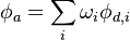 | (1) |
 is the value of the variable interpolated at the acceptor cell,
  are the values of the donor cells and
  are the weights with which the values of the donor cells
  are applied. In an overset mesh, donor and acceptor cells are on disconnected mesh zones. This means that they are not connected over a face and the standard connectivity between cells cannot be used to construct the matrix. In brief, the procedure how to achieve an overset interpolation in OpenFOAM is the following: 1) Extend the existing ldu adressing and 2) insert the coefficients resulting from the overset interpolation in the matrix and 3) solve the linear system.
A brief description of how a matrix is constructed in OpenFOAM using a finite volume discretization can be found here https://openfoamwiki.net/index.php/OpenFOAM_guide/Matrices_in_OpenFOAM.
3.1 Overset interpolation
Let's start to analyze how the ldu addressing in OpenFOAM is extended by the additional connectivity resulting from the overset interpolation. As first step let's recap how the connectivity between cells and the entries in the matrix in OpenFOAM are stored. The connectivity between the cells are stored in two arrays with the same length:
lowerAddr()
upperAddr()
In the
lowerAddr()
array the smaller index of the two coupled cells are stored and in the
upperAddr()
array the higher index of two coupled cells is stored. In OpenFOAM this both arrays have the length equal to the number of faces since only adjacent cells are used for the discretization.
The corresponding entries in the matrix are stored in other two arrays:
lower()
upper()
In order to account for the additional coupling between cell centers introduced by the overset meh approach, new entries in the matrix have to be accomplished. This means that the length of the above four arrays has to be enlarged. In the arrays
lowerAddr()
upperAddr()
the additional indexes of the cells coupled by the overset interpolation has to be added. In the arrays
lower()

upper()
the coefficients in the matrix resulting from the coupling have to be added. This is done during step when the mesh is updated:
bool changed = mesh.update();
In case of solvers which use the overset method, the mesh instance is of type dynamicOversetFvMesh. The method update can be found in dynamicOversetFvMesh.C:
bool Foam::dynamicOversetFvMesh::update()
{
    //if (dynamicMotionSolverFvMesh::update())
    if (dynamicMotionSolverListFvMesh::update())
    {
        // Calculate the local extra faces for the interpolation. Note: could
        // let demand-driven lduAddr() trigger it but just to make sure.
        updateAddressing();

        // Addressing and/or weights have changed. Make interpolated cells
        // up to date with donors
        interpolateFields();

        return true;
    }

    return false;
}
The updating of the addressing happens function fvMeshPrimitiveLduAddressing::addAddressing in the file fvMeshPrimitiveLduAddressing.C:
Foam::labelList Foam::fvMeshPrimitiveLduAddressing::addAddressing
(
    const lduAddressing& addr,
    const labelListList& nbrCells,
    label& nExtraFaces,
    labelList& newLowerAddr,
    labelList& newUpperAddr,
    labelListList& nbrCellFaces,
    const globalIndex& globalNumbering,
    const labelList& globalCellIDs,
    labelListList& localFaceCells,
    labelListList& remoteFaceCells
)
{
    label nCells = addr.size();
    label nFaces = addr.upperAddr().size();
    labelList nProcFaces(Pstream::nProcs(), Zero);

    // Count additional faces
    nExtraFaces = 0;
    forAll(nbrCells, cellI)
    {
        const labelList& nbrs = nbrCells[cellI];
        forAll(nbrs, nbrI)
        {
            if (nbrs[nbrI] < nCells)
            {
                // Local cell
                if (triIndex(addr, cellI, nbrs[nbrI]) == -1)
                {
                    nExtraFaces++;
                }
            }
            else
            {
                label globalNbr = globalCellIDs[nbrs[nbrI]];
                label procI = globalNumbering.whichProcID(globalNbr);
                nProcFaces[procI]++;
            }
        }
    }

    // Create space for extra addressing
    newLowerAddr.setSize(nFaces + nExtraFaces);
    newUpperAddr.setSize(nFaces + nExtraFaces);

    // Copy existing addressing
    SubList<label>(newLowerAddr, nFaces) = addr.lowerAddr();
    SubList<label>(newUpperAddr, nFaces) = addr.upperAddr();


    // Per processor its local cells we want
    localFaceCells.setSize(Pstream::nProcs());
    remoteFaceCells.setSize(Pstream::nProcs());
    forAll(nProcFaces, procI)
    {
        localFaceCells[procI].setSize(nProcFaces[procI]);
        remoteFaceCells[procI].setSize(nProcFaces[procI]);
    }
    nProcFaces = 0;

    nbrCellFaces.setSize(nbrCells.size());
    forAll(nbrCells, cellI)
    {
        const labelList& nbrs = nbrCells[cellI];
        labelList& faces = nbrCellFaces[cellI];
        faces.setSize(nbrs.size());

        forAll(nbrs, nbrI)
        {
            label nbrCellI = nbrs[nbrI];

            if (nbrCellI < nCells)
            {
                // Find neighbour cell in owner list
                label faceI = triIndex(addr, cellI, nbrCellI);
                if (faceI == -1)
                {
                    faceI = nFaces++;
                    newLowerAddr[faceI] = min(cellI, nbrCellI);
                    newUpperAddr[faceI] = max(cellI, nbrCellI);
                }
                faces[nbrI] = faceI;
            }
            else
            {
                // Remote cell
                faces[nbrI] = -1;

                label globalNbr = globalCellIDs[nbrCellI];
                label procI = globalNumbering.whichProcID(globalNbr);
                label remoteCellI = globalNumbering.toLocal(procI, globalNbr);

                label procFaceI = nProcFaces[procI]++;
                localFaceCells[procI][procFaceI] = cellI;
                remoteFaceCells[procI][procFaceI] = remoteCellI;
            }
        }
    }

    // Reorder upper-triangular
    labelList oldToNew
    (
        lduPrimitiveMesh::upperTriOrder
        (
            addr.size(),
            newLowerAddr,
            newUpperAddr
        )
    );

    // Shuffle face-to-cell addressing
    inplaceReorder(oldToNew, newLowerAddr);
    inplaceReorder(oldToNew, newUpperAddr);
    // Update cell-to-face addressing
    forAll(nbrCellFaces, cellI)
    {
        inplaceRenumber(oldToNew, nbrCellFaces[cellI]);
    }


    return oldToNew;
}
The information of the indices of the coupled cells is contained in the cellcellStencil object. It is basically a list of lists. For each index of the interpolated cells it contains the indices of the donor cell. If one knows the pairing index donor cell and acceptor cell, one can update the lduaddrissing. The lower index can be inserted in the lowerAddr array and the higer index can be inserted in the upperAdrr array. This is down by the following code snippet:
    if (nbrCellI < nCells)
            {
                // Find neighbour cell in owner list
                label faceI = triIndex(addr, cellI, nbrCellI);
                if (faceI == -1)
                {
                    faceI = nFaces++;
                    newLowerAddr[faceI] = min(cellI, nbrCellI);
                    newUpperAddr[faceI] = max(cellI, nbrCellI);
                }
                faces[nbrI] = faceI;
            }
4 References
- ↑ M. Breuer, G. De Nayer, M. Münsch, T. Gallinger, and R. Wüchner, “Fluid–structure interac tion using a partitioned semi-implicit predictor–corrector coupling scheme for the application of large-eddy simulation,” Journal of Fluids and Structures, vol. 29, pp. 107–130, 2012.
- ↑ W. J. Horne and K. Mahesh, “A massively-parallel, unstructured overset method to simulate moving bodies in turbulent flows,” Journal of Computational Physics, vol. 397, p. 108790, 2019.
- ↑ 2019. J. H. Ferziger, M. Perić, and R. L. Street, Computational methods for fluid dynamics. Springer, 2002, vol. 3.
- ↑ ] M. Buchmayr, Development of Fully Implicit Block Coupled Solvers for Incompressible Transient Flows. TU-Graz, 2014.
- ↑ mechanics, vol. 33, no. 1, pp. 445–490, 2001. H. Jasak, “Dynamic mesh handling in openfoam,” in 47th AIAA aerospace sciences meeting including the new horizons forum and aerospace exposition, 2009, p. 341.
- ↑ M. Breuer, G. De Nayer, M. Münsch, T. Gallinger, and R. Wüchner, “Fluid–structure interac tion using a partitioned semi-implicit predictor–corrector coupling scheme for the application of large-eddy simulation,” Journal of Fluids and Structures, vol. 29, pp. 107–130, 2012.