Difference between revisions of "Contrib/CompressibleMixingPhaseChangeFoam"
Mkraposhin (Talk | contribs) |
m (Wyldckat moved page CompressibleMixingPhaseChangeFoam to Contrib/CompressibleMixingPhaseChangeFoam: Was not within the defined contributions namespace) |
||
| (21 intermediate revisions by 2 users not shown) | |||
| Line 1: | Line 1: | ||
Solver for two fluids with phase change (for example - water <---> steam), pressure and temperature density dependence | Solver for two fluids with phase change (for example - water <---> steam), pressure and temperature density dependence | ||
| − | + | {{VersionInfo}}{{Version2.1.0}} | |
== Model Equations Derivation == | == Model Equations Derivation == | ||
| + | VALID OPENFOAM VERSION - 2.1.0 | ||
* '''Equation of state''' | * '''Equation of state''' | ||
Low-compressible fluid: <math> | Low-compressible fluid: <math> | ||
| Line 7: | Line 8: | ||
</math> | </math> | ||
| − | Ideal gas: <math> \rho=\frac{p}{ | + | Ideal gas: <math> \rho=\frac{p}{(R/M)T} |
</math> | </math> | ||
| Line 107: | Line 108: | ||
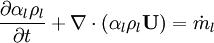
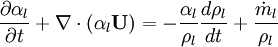
* '''Energy equation''' | * '''Energy equation''' | ||
| − | Energy equation for mixture temperature obtained from sum of energy equations for each phase. Consider energy equation for phase-1: | + | Energy equation for mixture temperature obtained from sum of energy equations for each phase. Consider internal energy equation for phase-1: |
<math> | <math> | ||
\frac{\partial \alpha_1 \rho_1 e_1} {\partial t} + | \frac{\partial \alpha_1 \rho_1 e_1} {\partial t} + | ||
| − | \nabla \cdot \left ( \alpha_1 \rho_1 e_1 \textbf{U} \right ) | + | \nabla \cdot \left ( \alpha_1 \rho_1 e_1 \textbf{U} \right ) + \nabla \cdot \textbf{q}_1 |
= | = | ||
| + | -\alpha_1 p (\nabla \cdot \textbf{U} - \dot m_1 / \rho_1) | ||
| + | + | ||
\dot m_1 e_1 | \dot m_1 e_1 | ||
</math> | </math> | ||
| − | |||
| − | + | By combining equations of phases, we get internal energy balance for mixture in temperatures: | |
| − | + | ||
| − | + | ||
| − | + | ||
| − | + | ||
| − | + | ||
| − | + | ||
| − | + | ||
| − | + | ||
| − | + | ||
| − | + | ||
| − | + | ||
| − | + | ||
| − | + | ||
| − | + | ||
| − | + | ||
| − | + | ||
| − | + | ||
| − | + | ||
| − | + | ||
| − | + | ||
| − | + | ||
| − | + | ||
| − | + | ||
| − | + | ||
| − | By combining equations of phases, we get energy balance for mixture: | + | |
<math> | <math> | ||
\frac{\partial T}{\partial t} + \nabla \cdot \left ( T \textbf{U} \right ) - T \nabla \cdot \textbf{U} | \frac{\partial T}{\partial t} + \nabla \cdot \left ( T \textbf{U} \right ) - T \nabla \cdot \textbf{U} | ||
| − | -\frac{1}{\rho_1 C_{ | + | -\frac{1}{\alpha_1 \rho_1 C_{v,1} + \alpha_2 \rho_2 C_{v,2}} (\nabla \cdot \kappa_1 \nabla T + \nabla \cdot \kappa_2 \nabla T) |
= | = | ||
</math> | </math> | ||
<math> | <math> | ||
| − | \left ( \frac{ | + | -\left ( \nabla \cdot \textbf{U} - \left(\frac{1}{\rho_1}-\frac{1}{\rho_2}\right) \dot m_1 \right ) |
| − | + | \frac{p}{\alpha_1 \rho_1 C_{v,1} + \alpha_2 \rho_2 C_{v,2}} | |
| − | + \ | + | - \left ( \frac{\partial L}{\partial t} + \nabla \cdot (\textbf{U} L) - L \nabla \cdot \textbf{U} \right ) |
| + | \frac{\alpha_2 \rho_2}{\alpha_1 \rho_1 C_{v,1} + \alpha_2 \rho_2 C_{v,2}} | ||
</math> | </math> | ||
| + | |||
| + | Where <math> L </math> - latent heat of evaporation | ||
* '''Linking liquid volume transport to pressure equation''' is done by introducing <math>+\alpha_1 \nabla \cdot \textbf{U}</math> and <math>-\alpha_1 \nabla \cdot \textbf{U}</math> at r.h.s of volume fraction balance equation. Then, <math>-\nabla \cdot \textbf{U}</math> replaced by value from pressure equation | * '''Linking liquid volume transport to pressure equation''' is done by introducing <math>+\alpha_1 \nabla \cdot \textbf{U}</math> and <math>-\alpha_1 \nabla \cdot \textbf{U}</math> at r.h.s of volume fraction balance equation. Then, <math>-\nabla \cdot \textbf{U}</math> replaced by value from pressure equation | ||
| Line 166: | Line 146: | ||
= | = | ||
\alpha_1 \nabla \cdot \textbf{U} + | \alpha_1 \nabla \cdot \textbf{U} + | ||
| − | \dot m_1 \left (\frac{1}{\rho_1} \alpha_1 | + | \dot m_1 \left (\frac{1}{\rho_1} - \alpha_1 \left (\frac{1}{\rho_1} - \frac{1}{\rho_2} \right ) \right ) + |
</math> | </math> | ||
| Line 175: | Line 155: | ||
</math> | </math> | ||
| − | * Phase change model | + | == Implemented phase change models == |
| + | * Phase change model Schnerr-Sauer | ||
| + | * Phase change model Zwart | ||
| + | * Phase change model Singhal | ||
| + | * Phase change model Merkle | ||
| + | * Phase change model Kunz | ||
| + | |||
| + | == Model Source Code For OpenFOAM 2.1.0 == | ||
| + | [http://www.os-cfd.ru/compressibleMixingPhaseChangeFoam/compressibleMixingPhaseChangeFoam-New.tgz Source code for solver located here] | ||
| + | |||
| + | == Tutorial cases == | ||
| + | |||
| + | * '''Case #1 - cavitation on the hemispherical body''' | ||
| + | Problem description, initial and boundary conditions are shown on the figure | ||
| + | |||
| + | |||
| + | [[File:cavitator.jpg]] | ||
| + | '''Figure 1.1''' | ||
| + | |||
| + | Volume fraction of liquid (water) is shown on the next figure | ||
| + | [[File:H-alpha1.png]] | ||
| + | '''Figure 1.2''' | ||
| + | |||
| + | * '''Case #2 - hot water flashing in the nozzle''' | ||
| + | Problem description, initial and boundary conditions are shown on the figure 2.1 | ||
| + | |||
| + | |||
| + | [[File:Water-flashing.jpg]] | ||
| + | '''Figure 2.1''' | ||
| + | |||
| + | Volume and mass fractions of vapour are shown on the figures 2.2 and 2.3 | ||
| + | Pressure distribution is shown on figure 2.4 | ||
| + | Velocity magnitude and Mach number for compressible case are shown on figures 2.5 and 2.6 | ||
| + | Velocity magnitude for incompressible case is shown on the case 2.7 | ||
| + | Temperature distribution is located of figure 2.8 | ||
| + | |||
| + | [[File:f-alpha2.png]] | ||
| + | '''Figure 2.2''' | ||
| + | |||
| + | |||
| + | [[File:f-X2.png]] | ||
| + | '''Figure 2.3''' | ||
| + | |||
| + | |||
| + | [[File:f-pprofile.png]] | ||
| + | '''Figure 2.4''' | ||
| + | |||
| + | |||
| + | [[File:f-magU.png]] | ||
| + | '''Figure 2.5''' | ||
| + | |||
| + | |||
| + | [[File:f-Mach.png]] | ||
| + | '''Figure 2.6''' | ||
| + | |||
| + | |||
| + | [[File:f-magU-ico.png]] | ||
| + | '''Figure 2.7''' | ||
| + | |||
| + | |||
| + | [[File:f-T.png]] | ||
| + | '''Figure 2.8''' | ||
| − | + | [[Category:Multiphase flow solvers]] | |
| − | [ | + | |
Latest revision as of 19:45, 21 March 2015
Solver for two fluids with phase change (for example - water <---> steam), pressure and temperature density dependence
Valid versions: ![]()
Contents
1 Model Equations Derivation
VALID OPENFOAM VERSION - 2.1.0
- Equation of state
Low-compressible fluid: 
Ideal gas: 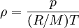
By combining this equations, we can get general relation:
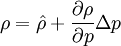
where  computed with respect to previous formulations
mixture density  calculated as
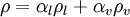
Here, and afterthere indices:
1,l,f - for liquid (heavy media with low compressibility)
2,g,s - for gas (light media (like steam) with big compressibility)
without index - mixture variable (or all variables local to some phase)
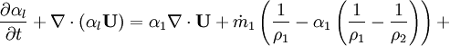
- Liquid volume transport
Let us consider transport of liquid (heavy phase) volume fraction  :
:
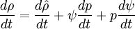
By converting to volume fluxes we get:
Using equation of state, we can reformulate substantial derivative for density in terms of pressure for any phase:
- General rule for converting from mass to volume fluxes in transport equation

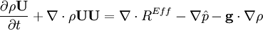
- Momentum equation (velocity prediction)
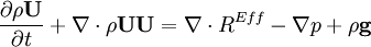
by substituting piezometric pressure 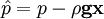 we get:
- Pressure equation obtained by summation of equation for volume phase fraction of liquid and gas phases:

- Energy equation
Energy equation for mixture temperature obtained from sum of energy equations for each phase. Consider internal energy equation for phase-1:

By combining equations of phases, we get internal energy balance for mixture in temperatures:


Where  - latent heat of evaporation
- Linking liquid volume transport to pressure equation is done by introducing
 and
and  at r.h.s of volume fraction balance equation. Then,
  replaced by value from pressure equation

2 Implemented phase change models
- Phase change model Schnerr-Sauer
- Phase change model Zwart
- Phase change model Singhal
- Phase change model Merkle
- Phase change model Kunz
3 Model Source Code For OpenFOAM 2.1.0
Source code for solver located here
4 Tutorial cases
- Case #1 - cavitation on the hemispherical body
Problem description, initial and boundary conditions are shown on the figure
 Figure 1.1
Volume fraction of liquid (water) is shown on the next figure
 Figure 1.2
- Case #2 - hot water flashing in the nozzle
Problem description, initial and boundary conditions are shown on the figure 2.1
 Figure 2.1
Volume and mass fractions of vapour are shown on the figures 2.2 and 2.3 Pressure distribution is shown on figure 2.4 Velocity magnitude and Mach number for compressible case are shown on figures 2.5 and 2.6 Velocity magnitude for incompressible case is shown on the case 2.7 Temperature distribution is located of figure 2.8
 Figure 2.2
 Figure 2.3
 Figure 2.4
 Figure 2.5
 Figure 2.6
 Figure 2.7
 Figure 2.8